Regla de la Cadena y Ecuaciones Parametricas
Regla de la Cadena y Ecuaciones Parametricas
Regla de la Cadena y Ecuaciones Parametricas

Create successful ePaper yourself
Turn your PDF publications into a flip-book with our unique Google optimized e-Paper software.
CALCULO DIFERENCIAL<br />
3.1. REGLA DE LA CADENA Y ECUACIONES<br />
PARAMETRICAS.<br />
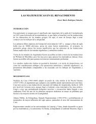
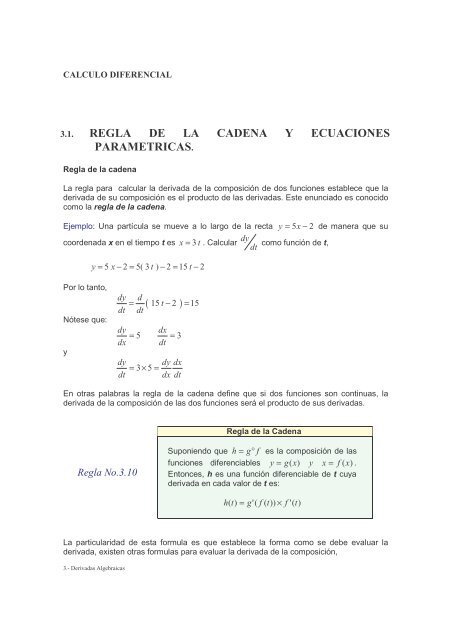
<strong>Reg<strong>la</strong></strong> <strong>de</strong> <strong>la</strong> ca<strong>de</strong>na<br />
La reg<strong>la</strong> para calcu<strong>la</strong>r <strong>la</strong> <strong>de</strong>rivada <strong>de</strong> <strong>la</strong> composición <strong>de</strong> dos funciones establece que <strong>la</strong><br />
<strong>de</strong>rivada <strong>de</strong> su composición es el producto <strong>de</strong> <strong>la</strong>s <strong>de</strong>rivadas. Este enunciado es conocido<br />
como <strong>la</strong> reg<strong>la</strong> <strong>de</strong> <strong>la</strong> ca<strong>de</strong>na.<br />
Ejemplo: Una partícu<strong>la</strong> se mueve a lo <strong>la</strong>rgo <strong>de</strong> <strong>la</strong> recta y = 5x − 2 <strong>de</strong> manera que su<br />
coor<strong>de</strong>nada x en el tiempo t es x = 3 t<br />
dy<br />
. Calcu<strong>la</strong>r como función <strong>de</strong> t,<br />
dt<br />
Por lo tanto,<br />
Nótese que:<br />
y<br />
y = 5 x − 2 = 5( 3 t ) − 2 = 15 t − 2<br />
3.- Derivadas Algebraicas<br />
dy d<br />
= ( 15 t − 2 ) = 15<br />
dt dt<br />
dy<br />
dx<br />
dy<br />
dt<br />
dx<br />
= 5 = 3<br />
dt<br />
= 3 × 5<br />
=<br />
dy dx<br />
dx dt<br />
En otras pa<strong>la</strong>bras <strong>la</strong> reg<strong>la</strong> <strong>de</strong> <strong>la</strong> ca<strong>de</strong>na <strong>de</strong>fine que si dos funciones son continuas, <strong>la</strong><br />
<strong>de</strong>rivada <strong>de</strong> <strong>la</strong> composición <strong>de</strong> <strong>la</strong>s dos funciones será el producto <strong>de</strong> sus <strong>de</strong>rivadas.<br />
<strong>Reg<strong>la</strong></strong> No.3.10<br />
<strong>Reg<strong>la</strong></strong> <strong>de</strong> <strong>la</strong> Ca<strong>de</strong>na<br />
Suponiendo que h = g°<br />
f es <strong>la</strong> composición <strong>de</strong> <strong>la</strong>s<br />
funciones diferenciables y = g(<br />
x)<br />
y x = f ( x)<br />
.<br />
Entonces, h es una función diferenciable <strong>de</strong> t cuya<br />
<strong>de</strong>rivada en cada valor <strong>de</strong> t es:<br />
h ( t)<br />
= g'<br />
( f ( t))<br />
× f '(<br />
t)<br />
La particu<strong>la</strong>ridad <strong>de</strong> esta formu<strong>la</strong> es que establece <strong>la</strong> forma como se <strong>de</strong>be evaluar <strong>la</strong><br />
<strong>de</strong>rivada, existen otras formu<strong>la</strong>s para evaluar <strong>la</strong> <strong>de</strong>rivada <strong>de</strong> <strong>la</strong> composición,
CALCULO DIFERENCIAL<br />
Otra es,<br />
3.- Derivadas Algebraicas<br />
dy<br />
dt<br />
t<br />
=<br />
dy<br />
dx<br />
f ( t)<br />
dx<br />
dt<br />
dy<br />
=<br />
dt<br />
Demostración <strong>de</strong> <strong>la</strong> <strong>Reg<strong>la</strong></strong> <strong>de</strong> <strong>la</strong> Ca<strong>de</strong>na<br />
t<br />
dy dx<br />
dx dt<br />
Si x =<br />
Δ x<br />
f (t)<br />
es diferenciable en t0 entonces un incremento Δ t produce otro incremento<br />
tal que:<br />
x = f '( t ) Δt<br />
+ ε Δt<br />
= f ' t + ε Δ<br />
[ ( ) ] t<br />
Δ 0<br />
1<br />
0 1<br />
y, si y = g(x)<br />
es diferenciable en x = f ( t0<br />
) entonces un incremento Δ x produce otro<br />
incremento Δy tal que:<br />
y = g'(<br />
x ) Δx<br />
+ ε Δx<br />
= g'<br />
x + ε Δ<br />
[ ( ) ] x<br />
Δ 0<br />
2<br />
0 2<br />
Estas dos ecuaciones re<strong>la</strong>cionan los incrementos Δ x y Δy<br />
con sus aproximaciones <strong>de</strong><br />
<strong>la</strong> recta tangente, en estas ecuaciones 1 0 → ε . cuando 0 → Δt , y 2 0 → ε cuando<br />
Δx → 0 .<br />
Combinando estas dos ecuaciones se tiene:<br />
[ g'<br />
( x ) + ε ] Δx<br />
= [ g'<br />
( x ) + ε ] [ f '(<br />
t ) + ε ] t<br />
Δ 0 2<br />
0 2 0 1<br />
y =<br />
Δ<br />
Dividiendo todo por Δ t<br />
Δy<br />
= [ g'<br />
( x0<br />
) + ε 2 ] [ f '(<br />
t0<br />
) + ε1<br />
]<br />
Δt<br />
Δy<br />
= g'(<br />
x0<br />
) f '(<br />
t0<br />
) + ε 2 f '(<br />
t0<br />
) + ε1g<br />
'(<br />
x0<br />
) + ε1ε<br />
2<br />
Δt<br />
Cuando → 0<br />
Ejemplo:<br />
Hal<strong>la</strong>r dy dt<br />
Δt , también lo hacen 1 2 , , ε y ε x<br />
Δ , y resulta:<br />
Δy<br />
Lim = g'<br />
0 0<br />
0 t<br />
Δt→0<br />
Δt<br />
en 1<br />
( x ) f '(<br />
t ) = g'(<br />
f ( t ) ) f '(<br />
)<br />
t = − , si: ( ) 3<br />
g x y x 5x 4<br />
= = + − , y ( ) 2<br />
0<br />
f t = x = t +<br />
t
CALCULO DIFERENCIAL<br />
Según <strong>la</strong> expresión :<br />
Ejercicios :<br />
3.- Derivadas Algebraicas<br />
dy<br />
dt<br />
t<br />
dy dx<br />
= , se tiene:<br />
dx dt<br />
f ( t)<br />
t<br />
dy dy dx<br />
= = 3 + 5 2 + 1 = 5 − 1 = − 5<br />
2 ( x ) ( t ) ( )( )<br />
0<br />
t 1<br />
dt x<br />
t 1 dx x f ( 1) dt =<br />
=−<br />
= = − t=−1<br />
= + 2 ( ) 100<br />
3<br />
y = x − 1<br />
2<br />
1 f ( x) x 1<br />
3 ( ) ( ) 4<br />
5<br />
y = 2x + 1<br />
3<br />
x − x + 1 4 ( ) ( ) 3<br />
4 2<br />
y = 2x − 5 8x − 5<br />
5<br />
2<br />
y = ( x + 1 ) 3 2<br />
x + 2<br />
6 ( ) 7<br />
3<br />
y = x + 4x<br />
7<br />
1<br />
y = t −<br />
t<br />
9 s ( t)<br />
=<br />
4<br />
t<br />
t<br />
3 2<br />
3<br />
3<br />
+ 1<br />
−1<br />
<strong>Ecuaciones</strong> Paramétricas<br />
8<br />
y =<br />
f z<br />
10 ( ) 5<br />
1<br />
( ) 4<br />
2<br />
t − 2t − 5<br />
=<br />
1<br />
2z − 1<br />
P , <strong>de</strong> <strong>la</strong><br />
curva en función <strong>de</strong> x, frecuentemente es más conveniente expresar ambas coor<strong>de</strong>nadas<br />
en función <strong>de</strong> una tercera variable.<br />
En lugar <strong>de</strong> escribir una curva expresando <strong>la</strong> coor<strong>de</strong>nada y <strong>de</strong> un punto ( x y)<br />
x = f (t)<br />
y = g(t)<br />
Esta ecuaciones se conocen con el nombre <strong>de</strong> ecuaciones Paramétricas y <strong>la</strong> variable t<br />
es conocida como el parámetro.<br />
dy dy dx<br />
=<br />
dt dx dt<br />
Expresión que también pue<strong>de</strong> expresarse como:<br />
dy<br />
=<br />
dt<br />
dy dt<br />
dx dt<br />
Lo anterior implica resolver <strong>la</strong> <strong>de</strong>rivada <strong>de</strong> cada una <strong>de</strong> <strong>la</strong>s funciones con re<strong>la</strong>ción al<br />
parámetro.<br />
−
CALCULO DIFERENCIAL<br />
d<br />
dt<br />
Ejemplo:<br />
( g(<br />
t))<br />
3.- Derivadas Algebraicas<br />
d<br />
y ( h(<br />
t))<br />
dt<br />
Dada <strong>la</strong> siguiente función <strong>de</strong>finida por <strong>la</strong>s ecuaciones paramétricas<br />
<strong>de</strong>terminar su <strong>de</strong>rivada.<br />
dx<br />
1 2t<br />
dt<br />
dy<br />
t<br />
dt<br />
dy<br />
2<br />
dy dt ( 1− 3t<br />
)<br />
= =<br />
dx dx ( 1− 2t<br />
)<br />
dt<br />
Derivadas segundas en forma Paramétrica:<br />
Si se tiene que:<br />
x = f (t)<br />
y = g(<br />
t)<br />
= g(<br />
h(<br />
t))<br />
= − Derivando a x<br />
2<br />
= 1− 3 Derivando a y<br />
Por <strong>de</strong>finición.<br />
2<br />
x = t − t y<br />
3<br />
y = t − t ,<br />
Definen a y como una función <strong>de</strong> x dos veces diferenciable, entonces es posible calcu<strong>la</strong>r:<br />
dy dy dt<br />
= y'<br />
=<br />
dx dx dt<br />
lo que permite <strong>de</strong>finir <strong>la</strong> segunda <strong>de</strong>rivada como:<br />
2<br />
d y dy´<br />
dy´<br />
dt<br />
= =<br />
2<br />
dx dx dx dt<br />
Esta ecuación permite expresar <strong>la</strong> segunda <strong>de</strong>rivada <strong>de</strong> y con respecto a x<br />
2<br />
d y<br />
2 como:<br />
dx<br />
Ejemplo:<br />
1. Expresar y ´ =<br />
dy<br />
en función <strong>de</strong> t.<br />
dx<br />
2.<br />
dy<br />
Diferenciar respecto a t.<br />
dx<br />
3. Dividir el resultado por dx<br />
dt<br />
Continuando con el ejemplo anterior, <strong>la</strong> segunda <strong>de</strong>rivada será:
CALCULO DIFERENCIAL<br />
1. Expresar<br />
3.- Derivadas Algebraicas<br />
y′<br />
=<br />
2 ( 1− 3t<br />
)<br />
( 1− 2t<br />
)<br />
2. Derivar y′ con respecto a t:<br />
dy′ d<br />
=<br />
dt dt<br />
1− 3t 1− 2t 2<br />
( 1− 2t )( −6t) −( 1− 3t )( −2)<br />
2 − 6t + 6t<br />
= =<br />
2 2<br />
1− 2t 1− 2t<br />
2 2<br />
3. Dividir el resultado por dx<br />
dt<br />
2<br />
2 − 6 t + 6t<br />
dy′<br />
2<br />
d y dt ( 1− 2 t ) 2 − 6 t + 6 t<br />
= = =<br />
2<br />
3<br />
dx dx ( 1− 2 t ) ( 1− 2 t<br />
dt<br />
)<br />
2 2<br />
Ejercicios Propuestos<br />
1. Hal<strong>la</strong>r dz , si<br />
dx<br />
2. Hal<strong>la</strong>r dy dx si<br />
( ) ( )<br />
2 1<br />
z w w −<br />
= − y w = 3 x<br />
y v v −<br />
3. Hal<strong>la</strong>r dr dt , si ( ) 1 2 r = s + 1 y<br />
v = 3 x + 2<br />
3 3<br />
= 2 + 2 y ( ) 2 3<br />
2<br />
16 20<br />
s = t − t<br />
3<br />
= 7 − 2 , y r = 1−<br />
1<br />
4. Hal<strong>la</strong>r da , si a<br />
db<br />
r<br />
b<br />
5. Hal<strong>la</strong>r dy , si 2 x − 3 y = 9 , y 2 x + t = 1<br />
dt 3<br />
6. Hal<strong>la</strong>r dy , si y x 2<br />
dt = + , y x = 2 , t 0<br />
t<br />
7. Hal<strong>la</strong>r dy , si<br />
dt<br />
8. Hal<strong>la</strong>r dy , si<br />
dt<br />
9. Hal<strong>la</strong>r<br />
2<br />
d y<br />
dx<br />
2<br />
4<br />
y = x , y<br />
x<br />
y =<br />
x<br />
, si<br />
2<br />
2<br />
+ 1<br />
, y 2 1<br />
2<br />
x = t − t , y<br />
3<br />
x = t<br />
x = t +<br />
3<br />
y = t −<br />
t