2º Regla de la cadena y derivación implícita
2º Regla de la cadena y derivación implícita
2º Regla de la cadena y derivación implícita

Create successful ePaper yourself
Turn your PDF publications into a flip-book with our unique Google optimized e-Paper software.
Capítulo 2<br />
<strong>Reg<strong>la</strong></strong> <strong>de</strong> <strong>la</strong> ca<strong>de</strong>na y <strong>de</strong>rivación<br />
<strong>implícita</strong><br />
En <strong>la</strong>s aplicaciones nos encontramos a menudo con <strong>la</strong> necesidad <strong>de</strong> usar<br />
funciones vectoriales <strong>de</strong> varias variables: una función vectorial <strong>de</strong> una variable<br />
<strong>de</strong>fine una curva, una función vectorial <strong>de</strong> tres componentes y dos variables<br />
<strong>de</strong>fine una superficie, una distribución <strong>de</strong> cargas eléctricas crea un campo<br />
eléctrico que se <strong>de</strong>scribe por medio <strong>de</strong> una función vectorial <strong>de</strong> tres com-<br />
ponentes y tres variables, etc. En este tema establecemos los conceptos <strong>de</strong><br />
función vectorial diferenciable y matriz jacobiana. El resultado fundamental<br />
es <strong>la</strong> reg<strong>la</strong> <strong>de</strong> <strong>la</strong> ca<strong>de</strong>na que nos muestra cómo se obtienen <strong>la</strong>s <strong>de</strong>rivadas par-<br />
ciales <strong>de</strong> una función compuesta f ◦ g en términos <strong>de</strong> <strong>la</strong>s <strong>de</strong>rivadas parciales<br />
<strong>de</strong> f y g. El tema termina con diversas aplicaciones <strong>de</strong> <strong>la</strong> reg<strong>la</strong> <strong>de</strong> <strong>la</strong> ca<strong>de</strong>na.<br />
2.1. Funciones vectoriales diferenciables.<br />
Sean f1, .., fm funciones <strong>de</strong>finidas en un subconjunto D <strong>de</strong> R n . La función<br />
<strong>de</strong>finida por<br />
x = (x1, .., xn) ∈ D → (f1(x), .., fm(x)) ∈ R m ,<br />
42
se dirá que es una función vectorial <strong>de</strong> n variables y m componentes y suele<br />
<strong>de</strong>notarse por f = (f1, .., fm). D es un subconjunto <strong>de</strong> R n que recibe el nombre<br />
<strong>de</strong> dominio <strong>de</strong> f.<br />
Ejemplo 2.1.1. El campo gravitatorio creado por una masa puntual m situ-<br />
ada en el origen viene dado por<br />
f(x, y, z) =<br />
<strong>de</strong>finido para (x, y, z) = (0, 0, 0).<br />
Gm<br />
(x2 + y2 + z2 (−x, −y, −z),<br />
) 3/2<br />
En este caso <strong>la</strong>s funciones componentes son<br />
f1(x, y, z) =<br />
f2(x, y, z) =<br />
f3(x, y, z) =<br />
−Gmx<br />
(x2 + y2 + z2 ,<br />
) 3/2<br />
−Gmy<br />
(x2 + y2 + z2 ,<br />
) 3/2<br />
−Gmz<br />
(x2 + y2 + z2 .<br />
) 3/2<br />
Diremos que una función vectorial f = (f1, .., fm) es diferenciable en un<br />
punto x0 cuando lo son todas sus componentes. Si f es diferenciable en x0,<br />
<strong>la</strong> matriz m × n cuyas fi<strong>la</strong>s son los gradientes <strong>de</strong> cada componente recibe el<br />
nombre <strong>de</strong> matriz jacobiana <strong>de</strong> f en el punto x0 y se <strong>de</strong>nota por f ′ (x0). Para<br />
facilitar <strong>la</strong> comprensión, vamos a <strong>de</strong>sarrol<strong>la</strong>r lo que resta <strong>de</strong> este apartado<br />
para el caso <strong>de</strong> funciones <strong>de</strong> dos variables y dos componentes.<br />
Si f = (f1, f2) es diferenciable en x0 = (x0, y0), sus dos componentes son<br />
diferenciables en dicho punto y, por tanto, existen los gradientes ∇fi(x0, y0)<br />
(i = 1, 2). La matriz jacobiana <strong>de</strong> f en el punto (x0, y0) tiene <strong>la</strong> forma<br />
f ′ <br />
∂f1<br />
∂x (x0, y0) =<br />
(x0,<br />
∂f1 y0) ∂y (x0,<br />
<br />
y0)<br />
∂f2<br />
∂x (x0, y0)<br />
∂f2<br />
∂y (x0, y0)<br />
Si necesitamos un valor aproximado <strong>de</strong> <strong>la</strong> diferencia<br />
f(x0 + ∆x, y0 + ∆y) − f(x0, y0),<br />
43
para valores pequeños <strong>de</strong> ∆x e ∆y, basta recordar que cada componente<br />
fi(x0 + ∆x, y0 + ∆y) − fi(x0, y0)<br />
<strong>de</strong> <strong>la</strong> diferencia vectorial anterior pue<strong>de</strong> aproximarse por<br />
dfi(x0, y0; ∆x, ∆y) = ∇fi(x0, y0) · (∆x, ∆y),<br />
puesto que cada fi es diferenciable en (x0, y0).<br />
Si <strong>de</strong>finimos <strong>la</strong> diferencial <strong>de</strong> <strong>la</strong> función vectorial por<br />
df(x0, y0; ∆x, ∆y) = (∆x, ∆y) · f ′ (x0, y0) t =<br />
<br />
∂f1<br />
∂f1<br />
t = (∆x, ∆y) ·<br />
∂x (x0, y0)<br />
∂f2<br />
∂x (x0, y0)<br />
∂y (x0, y0)<br />
∂f2<br />
∂y (x0, y0)<br />
entonces <strong>la</strong> diferencial es un vector cuyas componentes son aproximaciones<br />
<strong>de</strong> <strong>la</strong>s correspondientes componentes <strong>de</strong><br />
f(x0 + ∆x, y0 + ∆y) − f(x0, y0)<br />
y dichas aproximaciones son tanto mejores en cuanto los incrementos <strong>de</strong> <strong>la</strong>s<br />
variables in<strong>de</strong>pendientes, ∆x y ∆y, sean más pequeños.<br />
Ejemplo 2.1.2. Si f(x, y) = (xy, x 2 − y 2 ), estudiar si es diferenciable y<br />
calcu<strong>la</strong>r su diferencial.<br />
Sus componentes son <strong>la</strong>s funciones f1(x, y) = xy y f2(x, y) = x 2 − y 2 .<br />
Se trata <strong>de</strong> dos funciones que tienen <strong>de</strong>rivadas parciales <strong>de</strong> primer or<strong>de</strong>n<br />
continuas en R 2 y, por tanto, son diferenciables en cada punto <strong>de</strong> R 2 . Es-<br />
to <strong>de</strong>muestra que <strong>la</strong> función vectorial f es diferenciable en R 2 . La matriz<br />
jacobiana tiene <strong>la</strong> forma<br />
f ′ (x, y) =<br />
Entonces una aproximación <strong>de</strong><br />
<br />
44<br />
y x<br />
2x −2y<br />
<br />
.<br />
,
viene dada por<br />
f(x + ∆x, y + ∆y) − f(x, y)<br />
(∆x, ∆y) ·<br />
<br />
y x<br />
2x −2y<br />
t<br />
=<br />
= (y∆x + x∆y, 2x∆x − 2y∆y).<br />
El caso <strong>de</strong> funciones vectoriales <strong>de</strong> una variable real presenta una particu<strong>la</strong>ri-<br />
dad que <strong>de</strong>stacamos a continuación. El número <strong>de</strong> componentes es indiferente,<br />
pero, para simplificar, consi<strong>de</strong>raremos una función<br />
f : x ∈ I ⊂ R → f(x) = (f1(x), f2(x)) ∈ R 2 .<br />
Sus componentes f1 y f2 son funciones reales <strong>de</strong> variable real. Si x0 es un<br />
punto interior <strong>de</strong>l intervalo I, tiene sentido consi<strong>de</strong>rar el límite siguiente<br />
lím<br />
x→x0<br />
f(x) − f(x0)<br />
.<br />
x − x0<br />
Caso <strong>de</strong> existir, se <strong>de</strong>nota por f ′ (x0) y recibe el nombre <strong>de</strong> <strong>de</strong>rivada <strong>de</strong> f en<br />
el punto x0. Se trata <strong>de</strong> un vector <strong>de</strong> R 2 .<br />
Es fácil probar que el límite <strong>de</strong> una función vectorial es el vector cuyas<br />
componentes son los límites <strong>de</strong> cada componente <strong>de</strong> <strong>la</strong> función. Por tanto, en<br />
nuestro caso tenemos<br />
= lím<br />
x→x0<br />
f(x) − f(x0)<br />
lím<br />
x→x0 x − x0<br />
f1(x) − f1(x0)<br />
, lím<br />
x − x0 x→x0<br />
=<br />
f2(x) − f2(x0) <br />
.<br />
x − x0<br />
Vemos, pues, que f es <strong>de</strong>rivable en x0 cuando lo son sus componentes y<br />
se verifica f ′ (x0) = (f ′ 1(x0), f ′ 2(x0)). La matriz jacobiana <strong>de</strong> f es <strong>la</strong> matriz<br />
columna f ′ (x0) t = (f ′ 1(x0), f ′ 2(x0)) t . Entre funciones vectoriales <strong>de</strong> una vari-<br />
able, el concepto <strong>de</strong> <strong>de</strong>rivada <strong>de</strong> una función en un punto es <strong>de</strong> mayor interés<br />
45
y se usa más a menudo que el <strong>de</strong> matriz jacobiana; por ello, reservaremos <strong>la</strong><br />
notación<br />
f ′ (x0) = (f ′ 1(x0), f ′ 2(x0))<br />
para <strong>la</strong> <strong>de</strong>rivada <strong>de</strong> f en x0, mientras que <strong>la</strong> matriz jacobiana se <strong>de</strong>notará por<br />
f ′ (x0) t .<br />
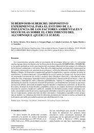
Una ecuación <strong>de</strong>l tipo x(t) = (x(t), y(t)), con t ∈ [a, b], pue<strong>de</strong> interpre-<br />
tarse como <strong>la</strong> ecuación paramétrica <strong>de</strong> una curva p<strong>la</strong>na. Vamos a mostrar que<br />
el vector <strong>de</strong>rivada x ′ (t0) es un vector tangente a <strong>la</strong> curva en el punto x(t0).<br />
En efecto, el cociente incremental<br />
x(t) − x(t0)<br />
,<br />
t − t0<br />
es un vector con igual dirección y sentido que x(t) − x(t0), si t > t0; en<br />
cambio, si t < t0, el sentido es el contrario.<br />
y<br />
O<br />
x(t )<br />
o<br />
x -x<br />
(t) (t o)<br />
x<br />
x(t)<br />
En cualquier caso, el cociente incremental es un vector paralelo a <strong>la</strong> cuerda<br />
<strong>de</strong> extremos x(t) y x(t0), y dirigido en el sentido en que x(t) recorre <strong>la</strong> curva.<br />
46<br />
x
Al tomar límite cuando t → t0, se obtiene un vector tangente a <strong>la</strong> curva en<br />
el punto x(t0) y dirigido en el sentido mencionado.<br />
Terminamos este apartado haciendo notar que <strong>la</strong> matriz jacobiana <strong>de</strong> una<br />
función esca<strong>la</strong>r no es otra cosa que el gradiente, y si <strong>la</strong> función esca<strong>la</strong>r es <strong>de</strong><br />
una só<strong>la</strong> variable, entonces <strong>la</strong> matriz jacobiana tiene un único elemento que<br />
es <strong>la</strong> <strong>de</strong>rivada ordinaria f ′ (x0).<br />
2.2. La reg<strong>la</strong> <strong>de</strong> <strong>la</strong> ca<strong>de</strong>na<br />
Sean f y g funciones reales <strong>de</strong> una variable ambas <strong>de</strong>rivables y tales que<br />
tiene sentido consi<strong>de</strong>rar <strong>la</strong> función compuesta g ◦ f. Al estudiar el cálculo<br />
diferencial <strong>de</strong> una variable vimos que <strong>la</strong> <strong>de</strong>rivada <strong>de</strong> g ◦f en x0 es el producto<br />
g ′ (f(x0)) · f ′ (x0). Es <strong>de</strong>cir, se verifica <strong>la</strong> igualdad<br />
(g ◦ f) ′ (x0) = g ′ (f(x0)) · f ′ (x0).<br />
La igualdad anterior suele <strong>de</strong>nominarse reg<strong>la</strong> <strong>de</strong> <strong>la</strong> ca<strong>de</strong>na. Esta reg<strong>la</strong> es<br />
válida para funciones <strong>de</strong> varias variables, esca<strong>la</strong>res o vectoriales. Si f y g son<br />
funciones diferenciables <strong>de</strong> cualquier número <strong>de</strong> variables, entonces<br />
(g ◦ f) ′ (x0) = g ′ (f(x0)) · f ′ (x0),<br />
don<strong>de</strong> el producto que aparece en el segundo miembro es el producto matricial<br />
<strong>de</strong> <strong>la</strong>s correspondientes matrices <strong>de</strong>rivadas.<br />
Para mayor c<strong>la</strong>ridad vamos a consi<strong>de</strong>rar dos <strong>de</strong> <strong>la</strong>s situaciones más co-<br />
munes con <strong>la</strong>s que nos encontraremos.<br />
I) Para facilitar <strong>la</strong> exposición, vamos a <strong>de</strong>notar <strong>la</strong>s variables in<strong>de</strong>pendi-<br />
entes por x1, x2 y x3. Supongamos que T (x1, x2, x3) es <strong>la</strong> temperatura en cada<br />
punto <strong>de</strong> una cierta región <strong>de</strong>l espacio y contenida en dicha región una curva<br />
dada por <strong>la</strong> ecuación<br />
x(t) = (x1(t), x2(t), x3(t))<br />
para t ∈ [a, b]. Nótese que T (x(t)) es el valor <strong>de</strong> <strong>la</strong> temperatura en el punto<br />
<strong>de</strong> <strong>la</strong> curva <strong>de</strong> coor<strong>de</strong>nadas (x1(t), x2(t), x3(t)). Si estuviéramos interesados<br />
47
en estudiar el comportamiento <strong>de</strong> <strong>la</strong> temperatura a lo <strong>la</strong>rgo <strong>de</strong> <strong>la</strong> curva,<br />
tendríamos que consi<strong>de</strong>rar <strong>la</strong> función compuesta T (x(t)).<br />
Ejemplo 2.2.1. Si T (x1, x2, x3) = x 2 1 + x 2 2 + x 2 3 y C es <strong>la</strong> curva <strong>de</strong> ecuaciones<br />
paramétricas<br />
x1 = cos t, x2 = sen t, x3 = t 2 ,<br />
entonces Tc(t) = cos 2 t + sen 2 t + t 4 = 1 + t 4 es <strong>la</strong> función que nos marca<br />
<strong>la</strong> temperatura en los puntos <strong>de</strong> <strong>la</strong> curva y no es otra cosa que <strong>la</strong> función<br />
compuesta T (x(t)).<br />
Continuando con el <strong>de</strong>sarrolo anterior, vamos a ver cómo se obtiene <strong>la</strong><br />
<strong>de</strong>rivada <strong>de</strong> <strong>la</strong> función temperatura sobre <strong>la</strong> curva, Tc(t) = T (x(t)), usando<br />
<strong>la</strong> reg<strong>la</strong> <strong>de</strong> <strong>la</strong> ca<strong>de</strong>na. Como T es una función esca<strong>la</strong>r, su matriz jacobiana es<br />
∇T y, recordando lo que acabamos <strong>de</strong> ver en el apartado anterior, x ′ (t0) t es<br />
<strong>la</strong> matriz jacobiana <strong>de</strong> x(t) en t0. Entonces <strong>la</strong> <strong>de</strong>rivada T ′ c(t0) viene dada por<br />
el producto matricial<br />
∇T (x(t0)) · (x ′ 1(t0), x ′ 2(t0), x ′ 3(t0)) t .<br />
Por tanto, hemos obtenido <strong>la</strong> igualdad<br />
dTc<br />
dt (t0) =<br />
3 ∂T<br />
i=1<br />
∂xi<br />
(x(t0)) · dxi<br />
dt (t0).<br />
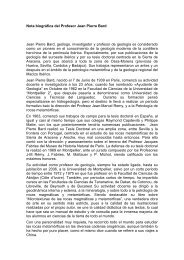
La expresión anterior conduce a <strong>la</strong> reg<strong>la</strong> práctica siguiente:<br />
En primer lugar, dibujamos un diagrama que exprese cómo <strong>de</strong>pen<strong>de</strong> Tc(t))<br />
<strong>de</strong> <strong>la</strong> variable t a través <strong>de</strong> <strong>la</strong>s variables x1, x2 y x3.<br />
48
T(x(t))<br />
T<br />
Vemos que hay tres caminos para llegar <strong>de</strong>s<strong>de</strong> T hasta t. Entonces<br />
dTc<br />
dt (t0)<br />
viene dada por una suma con tres sumandos. Cada sumando correspon<strong>de</strong><br />
a un camino. El sumando correspondiente al camino T → xi → t es un<br />
producto <strong>de</strong> <strong>la</strong> forma ∂T dxi · ∂xi dt .<br />
II) Cambios <strong>de</strong> variables.<br />
En <strong>la</strong>s aplicaciones nos encontramos a menudo con el problema <strong>de</strong> conocer<br />
cómo se re<strong>la</strong>cionan <strong>la</strong>s <strong>de</strong>rivadas parciales ∂T<br />
∂x<br />
x<br />
x<br />
x<br />
1<br />
2<br />
3<br />
y ∂T<br />
∂y<br />
con ∂T<br />
∂ρ<br />
t<br />
t<br />
t<br />
∂T y , para po<strong>de</strong>r<br />
∂ω<br />
<strong>de</strong>terminar <strong>la</strong> nueva ecuación a partir <strong>de</strong> <strong>la</strong> ecuación en cartesianas. Para<br />
ello, usaremos <strong>de</strong> nuevo <strong>la</strong> reg<strong>la</strong> <strong>de</strong> <strong>la</strong> ca<strong>de</strong>na.<br />
Ejemplo 2.2.2. De cierta magnitud T , que es función <strong>de</strong> otras dos x e y,<br />
se conoce que verifica cierta ecuación en <strong>de</strong>rivadas parciales respecto <strong>de</strong> <strong>la</strong>s<br />
coor<strong>de</strong>nadas po<strong>la</strong>res; por ejemplo, se sabe que T satisface <strong>la</strong> ecuación<br />
sen ω ∂T<br />
∂ρ<br />
+ cos ω<br />
ρ<br />
∂T<br />
∂ω<br />
= 0, (2.1)<br />
y se <strong>de</strong>sea encontrar <strong>la</strong> ecuación que verifica T respecto <strong>de</strong> <strong>la</strong>s coor<strong>de</strong>nadas<br />
cartesianas.<br />
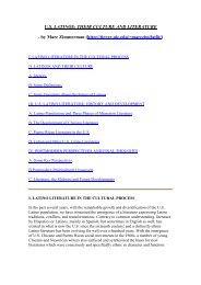
Primero vamos a proce<strong>de</strong>r haciendo uso <strong>de</strong> <strong>la</strong> reg<strong>la</strong> práctica y posteri-<br />
ormente usaremos <strong>la</strong> forma matricial. La reg<strong>la</strong> práctica nos dice que, para<br />
49
empezar, <strong>de</strong>bemos dibujar un diagrama que exprese <strong>la</strong> <strong>de</strong>pen<strong>de</strong>ncia <strong>de</strong> T<br />
respecto <strong>de</strong> <strong>la</strong>s coor<strong>de</strong>nadas po<strong>la</strong>res ρ y ω a través <strong>de</strong> x e y<br />
T<br />
x<br />
y<br />
Vemos que para llegar <strong>de</strong>s<strong>de</strong> T , tanto a ρ como a ω, hay dos caminos,<br />
pues x = ρ · cos ω e y = ρ · sen ω. Por tanto, cada <strong>de</strong>rivada parcial ∂T<br />
∂ρ y<br />
∂T<br />
∂ω<br />
consta <strong>de</strong> dos sumandos, uno por cada camino. Al camino T → x → ρ<br />
correspon<strong>de</strong> el sumando ∂T<br />
∂x<br />
sumando <strong>de</strong> <strong>la</strong> forma ∂T<br />
∂y<br />
· ∂y<br />
∂ρ<br />
∂T<br />
∂ρ<br />
∂T<br />
∂ω<br />
r<br />
w<br />
r<br />
w<br />
∂x · , mientras que el camino T → y → ρ aporta un<br />
∂ρ<br />
. En <strong>de</strong>finitiva, se tienen <strong>la</strong>s siguientes re<strong>la</strong>ciones<br />
= ∂T<br />
∂x<br />
= ∂T<br />
∂x<br />
∂x ∂T<br />
· +<br />
∂ρ ∂y<br />
∂x ∂T<br />
· +<br />
∂ω ∂y<br />
· ∂y<br />
∂ρ<br />
· ∂y<br />
∂ω .<br />
Pasamos ahora a obtener <strong>la</strong>s re<strong>la</strong>ciones anteriores haciendo uso <strong>de</strong> <strong>la</strong> ex-<br />
presión matricial <strong>de</strong> <strong>la</strong> reg<strong>la</strong> <strong>de</strong> <strong>la</strong> ca<strong>de</strong>na. Denotamos por g <strong>la</strong> función que<br />
cambia <strong>de</strong> coor<strong>de</strong>nadas<br />
(ρ, ω) ∈ (0, +∞) × [0, 2π] → (x, y) =<br />
= (ρ · cos ω, ρ · sen ω) ∈ R 2 .<br />
50
Nótese que <strong>la</strong> función compuesta (esca<strong>la</strong>r) T ◦ g es <strong>la</strong> que expresa T en<br />
coor<strong>de</strong>nadas po<strong>la</strong>res. La reg<strong>la</strong> <strong>de</strong> <strong>la</strong> ca<strong>de</strong>na nos dice que el producto matricial<br />
∇T · g ′ es el gradiente <strong>de</strong> <strong>la</strong> función compuesta; es <strong>de</strong>cir<br />
( ∂T ∂T<br />
) = (∂T<br />
∂ρ ∂ω ∂x<br />
<br />
∂x<br />
∂T ∂ρ ) ·<br />
∂y<br />
∂x<br />
∂ω<br />
<br />
.<br />
Terminamos este apartado resolviendo el problema p<strong>la</strong>nteado en el ejem-<br />
plo anterior. A partir <strong>de</strong> <strong>la</strong>s expresiones que hemos encontrado para ∂T<br />
∂ρ<br />
obtenemos<br />
sen ω ∂T<br />
∂ρ<br />
cos ω<br />
ρ<br />
∂T<br />
∂ω<br />
∂y<br />
∂ρ<br />
∂y<br />
∂ω<br />
= sen ω cos ω ∂T<br />
∂x + sen2 ω ∂T<br />
∂y<br />
= − cos ω sen ω ∂T<br />
∂x + cos2 ω ∂T<br />
∂y .<br />
Sumando <strong>la</strong>s dos igualda<strong>de</strong>s anteriores resulta<br />
sen ω ∂T<br />
∂ρ<br />
+ cos ω<br />
ρ<br />
∂T<br />
∂ω = (sen2 ω + cos 2 ω) ∂T<br />
∂y<br />
Por tanto, <strong>la</strong> ecuación en cartesianas se reduce a<br />
∂T<br />
∂y<br />
= 0.<br />
= ∂T<br />
∂y .<br />
2.3. P<strong>la</strong>no tangente a una superficie.<br />
y ∂T<br />
∂ω ,<br />
Consi<strong>de</strong>ramos <strong>la</strong> superficie <strong>de</strong> ecuación f(x, y, z) = 0 y vamos a pro-<br />
bar que, si (x0, y0, z0) es un punto <strong>de</strong> S, ∇f(x0, y0, z0) es un vector perpen-<br />
dicu<strong>la</strong>r al vector tangente, en dicho punto, a cualquier curva contenida en<br />
<strong>la</strong> superficie y que pasa por (x0, y0, z0). Sea, pues, x(t) = (x(t), y(t), z(t))<br />
(t ∈ [a, b]) <strong>la</strong> ecuación <strong>de</strong> una curva que está contenida en <strong>la</strong> superficie<br />
S y que pasa por el punto (x0, y0, z0). Entonces existe t0 ∈ [a, b] tal que<br />
x(t0) = (x(t0), y(t0), z(to)) y se verifica<br />
f(x(t), y(t), z(t)) = 0, para cada t ∈ [a, b].<br />
51
Por tanto, <strong>de</strong>rivando respecto <strong>de</strong> t, resulta para t = t0<br />
∇f(x(t0)) · x ′ (t0) t = 0,<br />
lo que prueba que ∇f(x0, y0, z0) y x ′ (t0) (el vector tangente a <strong>la</strong> curva en<br />
(x0, y0, z0)) son perpendicu<strong>la</strong>res.<br />
Ésta es <strong>la</strong> razón <strong>de</strong> que se <strong>de</strong>fina el p<strong>la</strong>no tangente a <strong>la</strong> superficie f(x, y, z) =<br />
0 en el punto (x0, y0, z0) como el p<strong>la</strong>no que pasa por dicho punto y es per-<br />
pendicu<strong>la</strong>r a ∇f(x0, y0, z0). Su ecuación tiene <strong>la</strong> forma<br />
∂f<br />
∂x · (x − x0) + ∂f<br />
∂y · (y − y0) + ∂f<br />
∂z · (z − z0) = 0,<br />
don<strong>de</strong> <strong>la</strong>s <strong>de</strong>rivadas parciales <strong>de</strong> f se toman en el punto (x0, y0, z0).<br />
Si <strong>la</strong> ecuación <strong>de</strong> <strong>la</strong> superficie viene dada en forma explícita por z =<br />
F (x, y), po<strong>de</strong>mos pasar a <strong>la</strong> forma explícita poniendo f(x, y, z) = F (x, y) −<br />
z = 0. De acuerdo con lo que acabamos <strong>de</strong> ver, el p<strong>la</strong>no tangente en el punto<br />
(x0, y0, F (x0, y0)) tiene por ecuación<br />
ya que ∂f<br />
∂x<br />
∂F<br />
∂x (x0, y0) · (x − x0) + ∂F<br />
∂y (x0, y0) · (y − y0)+<br />
∂F ∂f<br />
= , ∂x ∂y<br />
+(−1) · (z − F (x0, y0)) = 0,<br />
= ∂F<br />
∂y<br />
tangente adopta <strong>la</strong> forma final<br />
y ∂f<br />
∂z<br />
z = F (x0, y0) + ∂F<br />
∂x · (x − x0) + ∂F<br />
∂y<br />
= −1. Por tanto, <strong>la</strong> ecuación <strong>de</strong>l p<strong>la</strong>no<br />
· (y − y0),<br />
expresión que ya habiamos encontrado al estudiar el concepto <strong>de</strong> función<br />
diferenciable <strong>de</strong> dos variables.<br />
Ejemplo 2.3.1. Encontrar el p<strong>la</strong>no tangente a <strong>la</strong> superficie z = x 2 + y 2 en<br />
el punto (0, 0, 0).<br />
Calcu<strong>la</strong>mos <strong>la</strong>s <strong>de</strong>rivadas parciales <strong>de</strong> primer or<strong>de</strong>n z ′ x = 2x y z ′ y = 2y.<br />
Sus valores en el punto en cuestión son z ′ x(0, 0) = 0 y z ′ y(0, 0) = 0. Por tanto,<br />
<strong>la</strong> ecuación <strong>de</strong>l p<strong>la</strong>no tangente tiene <strong>la</strong> forma z = 0 + 0 · (x − 0) + 0 · (y − 0);<br />
es <strong>de</strong>cir, z = 0.<br />
52
Finalizamos el apartado <strong>de</strong>stacando una propiedad <strong>de</strong> ∇f en re<strong>la</strong>ción<br />
con <strong>la</strong>s superficies <strong>de</strong> nivel <strong>de</strong> f. Dada una función f <strong>de</strong> tres variables,<br />
f(x, y, z) = c es <strong>la</strong> ecuación <strong>de</strong> una superficie <strong>de</strong> nivel. Si (x0, y0, z0) es un<br />
punto <strong>de</strong> dicha superficie, <strong>de</strong>l mismo modo que hemos probado que ∇f es per-<br />
pendicu<strong>la</strong>r a <strong>la</strong> superficie f(x, y, z) = 0, pue<strong>de</strong> <strong>de</strong>mostrarse que ∇f(x0, y0, z0)<br />
es perpendicu<strong>la</strong>r a <strong>la</strong> superficie <strong>de</strong> nivel.<br />
2.4. El jacobiano<br />
En este apartado consi<strong>de</strong>ramos funciones vectoriales con n variables y<br />
n componentes. En tal caso, <strong>la</strong> matriz jacobiana es una matriz cuadrada<br />
<strong>de</strong> or<strong>de</strong>n n y tiene sentido calcu<strong>la</strong>r su <strong>de</strong>terminante que recibe el nombre<br />
<strong>de</strong> jacobiano <strong>de</strong> <strong>la</strong> función en el punto en cuestión. Más precisamente, si<br />
f : D ⊂ R n → R n es diferenciable en x0 ∈ D, el jacobiano <strong>de</strong> f en x0 es el<br />
<strong>de</strong>terminante <strong>de</strong> <strong>la</strong> matriz f ′ (x0) y se <strong>de</strong>nota por<br />
<strong>de</strong>t(f ′ (x0)) = ∂(f1, · · · , fn)<br />
∂(x1, · · · , xn) (x0).<br />
Si y = f(x), entonces también suele usarse <strong>la</strong> notación<br />
∂y<br />
∂r<br />
∂(y1, · · · , yn)<br />
∂(x1, · · · , xn) (x0).<br />
Ejemplo 2.4.1. Si x = r cos ω e y = r sen ω, entonces<br />
∂(x, y)<br />
∂(r, ω) =<br />
<br />
<br />
<br />
<br />
<br />
∂x<br />
∂r<br />
∂x<br />
∂ω<br />
<br />
<br />
<br />
<br />
=<br />
<br />
<br />
cos ω<br />
<br />
sen ω<br />
<br />
−r sen ω<br />
<br />
<br />
= r.<br />
r cos ω <br />
∂y<br />
∂ω<br />
En este caso, <strong>la</strong> función vectorial es <strong>la</strong> <strong>de</strong>finida por<br />
(r, ω) ∈ (0, +∞) × [0, 2π) → (x, y) =<br />
= (r cos ω, r sen ω) ∈ R 2 ,<br />
<strong>de</strong> dos componentes, x = r cos ω e y = r sen ω, y dos variables r y ω.<br />
53
Las dos propieda<strong>de</strong>s fundamentales <strong>de</strong>l jacobiano son <strong>la</strong>s siguientes:<br />
1) Si f es diferenciable en x0 y g lo es en f(x0), entonces el jacobiano <strong>de</strong> <strong>la</strong><br />
función compuesta g ◦ f es el producto <strong>de</strong> los jacobianos, es <strong>de</strong>cir, se verifica<br />
don<strong>de</strong> z = g(y) e y = f(x).<br />
∂(z1, · · · , zn)<br />
∂(x1, · · · , xn) = ∂(z1, · · · , zn)<br />
∂(y1, · · · , yn) · ∂(y1, · · · , yn)<br />
∂(x1, · · · , xn) ,<br />
2) Si f posee inversa diferenciable, entonces se verifica<br />
don<strong>de</strong> y = f(x).<br />
∂(y1, · · · , yn)<br />
∂(x1, · · · , xn) · ∂(x1, · · · , xn)<br />
∂(y1, · · · , yn)<br />
= 1,<br />
Ambas propieda<strong>de</strong>s se <strong>de</strong>ducen fácilmente a partir <strong>de</strong> <strong>la</strong> reg<strong>la</strong> <strong>de</strong> <strong>la</strong> ca-<br />
<strong>de</strong>na y <strong>de</strong>l hecho bien conocido <strong>de</strong> que el <strong>de</strong>terminante <strong>de</strong> un producto <strong>de</strong><br />
dos matrices es el producto <strong>de</strong> los <strong>de</strong>terminantes <strong>de</strong> ambas. En el caso <strong>de</strong> <strong>la</strong><br />
primera propiedad, <strong>la</strong> prueba proce<strong>de</strong>ría como sigue: <strong>la</strong> reg<strong>la</strong> <strong>de</strong> <strong>la</strong> ca<strong>de</strong>na<br />
nos dice que <strong>la</strong> matriz jacobiana <strong>de</strong> <strong>la</strong> función compuesta g ◦ f es el producto<br />
<strong>de</strong> <strong>la</strong>s matrices jacobianas <strong>de</strong> <strong>la</strong>s funciones g y f. Por tanto, el jacobiano <strong>de</strong> <strong>la</strong><br />
función compuesta es el <strong>de</strong>terminante <strong>de</strong> <strong>la</strong> matriz que resulta <strong>de</strong> multiplicar<br />
<strong>la</strong>s matrices jacobianas g ′ (f(x0)) y f ′ (x0), que es el producto <strong>de</strong> los <strong>de</strong>termi-<br />
nantes <strong>de</strong> ambas. Por lo que se refiere a 2), nótese que es consecuencia directa<br />
<strong>de</strong> <strong>la</strong> primera ya que f ◦ f −1 es <strong>la</strong> función i<strong>de</strong>ntidad cuya matriz jacobiana es<br />
<strong>la</strong> matriz unidad y, por tanto, su jacobiano es 1.<br />
Ejemplo 2.4.2. Sean u = y/x y v = x2 + y2 , calcu<strong>la</strong>r ∂(x,y)<br />
∂(u,v) .<br />
Lo más cómodo es calcu<strong>la</strong>r el jacobiano ∂(u,v)<br />
∂(x,y)<br />
resultado obtenido:<br />
∂(u, v)<br />
∂(x, y) =<br />
<br />
<br />
−y/x<br />
<br />
<br />
2 2x<br />
<br />
1/x<br />
<br />
<br />
<br />
2y <br />
y <strong>de</strong>spués invertimos el<br />
= −2y2<br />
x 2 − 2 = −2(u2 + 1).<br />
−1<br />
Entonces el jacobiano que buscamos es igual a 2(u2 , por <strong>la</strong> propiedad se-<br />
+1)<br />
gunda. Un cálculo sencillo permite obtener <strong>la</strong>s variables x e y en función <strong>de</strong><br />
54
u y v. Concretamente, x = v<br />
1+u2 e y = u v<br />
1+u2 . Con estas expresiones <strong>de</strong><br />
x e y, ahora podríamos obtener el jacobiano ∂(x,y)<br />
directamente, pero es más<br />
∂(u,v)<br />
simple el camino que hemos seguido consistente en calcu<strong>la</strong>r el jacobiano <strong>de</strong><br />
<strong>la</strong> función inversa para <strong>de</strong>spués aplicar <strong>la</strong> propiedad (2).<br />
2.5. Derivación <strong>implícita</strong>.<br />
Una ecuación <strong>de</strong>l tipo F (x, y) = 0 pue<strong>de</strong> interpretarse como <strong>la</strong> ecuación<br />
en forma <strong>implícita</strong> <strong>de</strong> una curva en el p<strong>la</strong>no OXY, ya que el conjunto <strong>de</strong><br />
los puntos que verifican <strong>la</strong> ecuación posee un grado <strong>de</strong> libertad (se pue<strong>de</strong>n<br />
escoger los valores <strong>de</strong> x libremente y los <strong>de</strong> y quedan <strong>de</strong>terminados por <strong>la</strong><br />
ecuación). Pero pue<strong>de</strong>n darse situaciones muy diversas como muestran los<br />
ejemplos siguientes.<br />
Ejemplos 2.5.1. a) F (x, y) = x 2 + e y = 0. En este caso <strong>la</strong> ecuación no tiene<br />
ninguna solución.<br />
b) F (x, y) = x 2 + y 2 = 0. Sólo el punto (0, 0) es solución.<br />
c) F (x, y) = e y − x 2 − 1 = 0. En este caso pue<strong>de</strong> <strong>de</strong>spejarse y y se obtiene<br />
y(x) = log(x 2 + 1).<br />
d) F (x, y) = x 2 +y 2 −1 = 0. Ahora también po<strong>de</strong>mos <strong>de</strong>spejar <strong>la</strong> variable<br />
y, pero obtenemos dos funciones diferentes y(x) = ± √ 1 − x 2 .<br />
Vemos que sólo en el ejemplo (c) <strong>la</strong> ecuación F (x, y) = 0 <strong>de</strong>fine im-<br />
plícitamente <strong>de</strong> una única manera a <strong>la</strong> variable y como función <strong>de</strong> x. En el<br />
ejemplo (d) <strong>la</strong> ecuación <strong>de</strong>fine <strong>implícita</strong>mente a y como función <strong>de</strong> x <strong>de</strong> dos<br />
formas diferentes. Hay una forma <strong>de</strong> conseguir que también en este ejemplo<br />
<strong>la</strong> ecuación <strong>de</strong>fina <strong>de</strong> forma única a y como función <strong>de</strong> x. Consiste en exigir<br />
que <strong>la</strong> función y(x) tome un valor pre<strong>de</strong>terminado para cierto valor <strong>de</strong> x. Por<br />
ejemplo, si queremos que y(0) = 1, entonces <strong>la</strong> ecuación x 2 +y 2 −1 = 0 <strong>de</strong>fine<br />
<strong>implícita</strong>mente a y como función <strong>de</strong> x <strong>de</strong> una única manera: y(x) = √ 1 − x 2 .<br />
El siguiente ejemplo pone <strong>de</strong> manifiesto <strong>la</strong> importancia que pue<strong>de</strong> tener<br />
este hecho.<br />
55
Ejemplo 2.5.2. Calcu<strong>la</strong>r lím<br />
0, y f(x, −x) = 0, para cada x ∈ R.<br />
(x,y)→(0,0) f(x, y), siendo f(x, y) = x3 +y3 x+y<br />
Primero vamos a calcu<strong>la</strong>r los límites a través <strong>de</strong> <strong>la</strong>s rectas y = mx<br />
lím<br />
(x, y) → (0, 0)<br />
y = mx<br />
x<br />
f(x, y) = lím<br />
x→0<br />
3 (1 + m3 )<br />
x(1 + m) =<br />
x<br />
= lím<br />
x→0<br />
2 (1 + m3 )<br />
(1 + m)<br />
= 0,<br />
, si x + y =<br />
si m = −1. Por otra parte, es c<strong>la</strong>ro que el límite a través <strong>de</strong> <strong>la</strong> recta y = −x<br />
también es 0. Ahora vamos a consi<strong>de</strong>rar <strong>la</strong> curva <strong>de</strong> ecuación F (x, y) =<br />
x 3 + y 3 − x − y = 0. Nótese que pasa por el punto (0, 0) y que en cada uno <strong>de</strong><br />
sus puntos f toma el valor constante 1. Por tanto, el límite <strong>de</strong> f a lo <strong>la</strong>rgo <strong>de</strong><br />
esta curva es igual a 1. Esto prueba que no existe el límite doble <strong>de</strong> f(x, y)<br />
en el origen pues <strong>la</strong> función es osci<strong>la</strong>nte en <strong>la</strong>s proximida<strong>de</strong>s <strong>de</strong> (0, 0). Pero<br />
hemos pasado por alto algo muy importante ¿cómo po<strong>de</strong>mos estar seguros<br />
<strong>de</strong> que <strong>la</strong> ecuación x 3 + y 3 − x − y = 0 <strong>de</strong>fine realmente una curva? Podría<br />
ocurrir, como en el ejemplo (b), que sólo el punto (0, 0) verificara <strong>la</strong> ecuación.<br />
En ese caso el razonamiento seguido para probar que no existe el límite doble<br />
se caería por su propio peso.<br />
El ejemplo muestra <strong>la</strong> importancia <strong>de</strong> disponer <strong>de</strong> un criterio práctico para<br />
<strong>de</strong>scubrir si, dados F (x, y) = 0 y un punto (x0, y0) tal que F (x0, y0) = 0, <strong>la</strong><br />
ecuación <strong>de</strong>fine <strong>implícita</strong>mente a y como función <strong>de</strong> x y esta función verifica<br />
que y(x0) = y0. El teorema siguiente muestra que se requiere <strong>la</strong> condición<br />
F ′ y(x0, y0) = 0.<br />
Teorema 2.5.3. (De <strong>la</strong> función <strong>implícita</strong>). Sea F una función <strong>de</strong> c<strong>la</strong>se uno<br />
en un entorno <strong>de</strong> (x0, y0) y tal que F (x0, y0) = 0 y F ′ y(x0, y0) = 0. Entonces<br />
existe un entorno E <strong>de</strong> x0 <strong>de</strong> modo que sólo hay una función y = y(x) <strong>de</strong>finida<br />
56
<strong>implícita</strong>mente en dicho entorno por <strong>la</strong> ecuación y verificando y(x0) = y0.<br />
A<strong>de</strong>más, esta función tiene <strong>de</strong>rivada continua en cada punto <strong>de</strong> E.<br />
Para terminar el ejemplo anterior, nótese que F ′ y(0, 0) = 3y 2 − 1|(0,0) =<br />
−1 = 0. De modo que queda garantizado que <strong>la</strong> ecuación F (x, y) = 0 <strong>de</strong>fine<br />
una curva que pasa por (0, 0).<br />
Supongamos que y = y(x) es una función <strong>de</strong>finida <strong>implícita</strong>mente por <strong>la</strong><br />
ecuación F (x, y) = 0 y queremos calcu<strong>la</strong>r y ′ (x). Vamos a ver que po<strong>de</strong>mos<br />
encontrar y ′ (x) aunque no dispongamos <strong>de</strong> <strong>la</strong> forma explícita <strong>de</strong> y(x). Basta<br />
observar que F (x, y(x)) = 0, para cada x ∈ D (D es el dominio <strong>de</strong> y(x)).<br />
Entonces <strong>la</strong> <strong>de</strong>rivada <strong>de</strong> F (x, y(x)) respecto <strong>de</strong> x es cero en D. Para obtener<br />
esta <strong>de</strong>rivada usaremos <strong>la</strong> reg<strong>la</strong> <strong>de</strong> <strong>la</strong> ca<strong>de</strong>na.<br />
<strong>de</strong> x.<br />
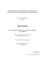
Primero dibujamos un diagrama que recoja <strong>la</strong> forma en que F <strong>de</strong>pen<strong>de</strong><br />
F<br />
x<br />
y x<br />
Hay dos formas <strong>de</strong> llegar <strong>de</strong>s<strong>de</strong> F a x, por lo que <strong>la</strong> <strong>de</strong>rivada <strong>de</strong> F (x, y(x))<br />
constará <strong>de</strong> dos sumandos.<br />
Al camino F → x le correspon<strong>de</strong> el sumando ∂F , mientras que al segundo<br />
∂x<br />
camino, F → y → x, correspon<strong>de</strong> un sumando <strong>de</strong> <strong>la</strong> forma ∂F<br />
∂y<br />
resulta<br />
para cada x ∈ D.<br />
∂F<br />
∂x<br />
+ ∂F<br />
∂y<br />
57<br />
· dy<br />
dx<br />
= 0,<br />
dy<br />
· . Por tanto,<br />
dx
Esta igualdad nos permite obtener<br />
y ′ ∂F<br />
∂x (x) = − , (2.2)<br />
∂F<br />
∂y<br />
expresión válida para cada x ∈ D tal que ∂F (x, y(x)) = 0.<br />
∂y<br />
Ejemplos 2.5.4. a) Encontrar <strong>la</strong> ecuación <strong>de</strong> <strong>la</strong> recta tangente a <strong>la</strong> circun-<br />
ferencia x 2 + y 2 = r 2 en el punto (x0, y0), siendo y0 > 0.<br />
Derivamos <strong>implícita</strong>mente en <strong>la</strong> ecuación x 2 + y 2 − r 2 = 0 y obtenemos<br />
2x + 2yy ′ = 0. Por tanto, y ′ (x0) = − x0 . Entonces <strong>la</strong> ecuación <strong>de</strong> <strong>la</strong> recta<br />
y0<br />
tangente viene dada por<br />
y − y0 = − x0<br />
(x − x0).<br />
Finalmente, como x 2 0 + y 2 0 = r 2 , <strong>la</strong> ecuación queda en <strong>la</strong> forma<br />
y0<br />
x0<br />
y − y0 = −<br />
(x − x0).<br />
r2 2 − x0 b) Calcu<strong>la</strong>r y ′ (0), siendo y(x) <strong>la</strong> única función <strong>implícita</strong> <strong>de</strong> x que <strong>de</strong>fine<br />
<strong>la</strong> ecuación F (x, y) = x 4 + y 4 + x 3 y − 1 = 0 en un entorno <strong>de</strong>l punto (0, 1).<br />
Es c<strong>la</strong>ro que F es una función <strong>de</strong> c<strong>la</strong>se uno en todo el p<strong>la</strong>no y que<br />
F (0, 1) = 0. Calcu<strong>la</strong>mos <strong>la</strong> <strong>de</strong>rivada parcial F ′ y(x, y) = 4y 3 + x 3 y <strong>la</strong> evalu-<br />
amos en el punto (0, 1): F ′ y(0, 1) = 4 = 0. Por tanto, el Teorema anterior<br />
nos garantiza que hay una función y(x) (única) <strong>de</strong>finida <strong>implícita</strong>mente por<br />
<strong>la</strong> ecuación en algún entorno <strong>de</strong>l origen y verificando y(0) = 1.<br />
Para <strong>de</strong>terminar su <strong>de</strong>rivada, po<strong>de</strong>mos emplear (2.2)<br />
Haciendo x = 0, obtenemos y ′ (0) = 0<br />
4<br />
ables:<br />
y ′ (x) = − F ′ x(x, y(x))<br />
F ′ y(x, y(x)) .<br />
= 0.<br />
Terminamos el tema consi<strong>de</strong>rando el caso <strong>de</strong> una ecuación <strong>de</strong> tres vari-<br />
58
F (x, y, z) = 0. Para saber si <strong>la</strong> ecuación <strong>de</strong>fine <strong>implícita</strong>mente a <strong>la</strong> variable<br />
z como función <strong>de</strong> <strong>la</strong>s variables x e y, en un entorno <strong>de</strong> un punto (x0, y0, z0)<br />
que verifica <strong>la</strong> ecuación, acudiremos a un Teorema simi<strong>la</strong>r al que acabamos<br />
<strong>de</strong> ver.<br />
Teorema 2.5.5. Sea F una función <strong>de</strong> c<strong>la</strong>se uno en un entorno <strong>de</strong> (x0, y0, z0)<br />
y tal que<br />
y<br />
F (x0, y0, z0) = 0<br />
F ′ z(x0, y0, z0) = 0.<br />
Entonces existe un entorno E <strong>de</strong> (x0, y0) <strong>de</strong> modo que sólo hay una función<br />
z = z(x, y) <strong>de</strong>finida <strong>implícita</strong>mente en dicho entorno por <strong>la</strong> ecuación y ver-<br />
ificando z(x0, y0) = z0. A<strong>de</strong>más, esta función tiene <strong>de</strong>rivadas parciales <strong>de</strong><br />
primer or<strong>de</strong>n continuas en cada punto <strong>de</strong> E.<br />
De hecho, existe un Teorema general <strong>de</strong> <strong>la</strong> función <strong>implícita</strong>, válido para<br />
una ecuación F (x1, .., xn, xn+1) = 0. En este caso, si se quiere que <strong>la</strong> ecuación<br />
<strong>de</strong>fina <strong>implícita</strong>mente a <strong>la</strong> variable xn+1 como función <strong>de</strong> <strong>la</strong>s restantes en un<br />
entorno <strong>de</strong>l punto x0, el Teorema exige que F ′ xn+1 no se anule en dicho punto.<br />
2.6. Sistemas <strong>de</strong> ecuaciones<br />
Consi<strong>de</strong>ramos el sistema <strong>de</strong> ecuaciones<br />
<br />
F (x, y, z) = 0<br />
G(x, y, z) = 0,<br />
(2.3)<br />
y nos p<strong>la</strong>nteamos <strong>la</strong> cuestión siguiente:¿qué condiciones <strong>de</strong>ben verificar F y<br />
G para que el sistema <strong>de</strong>fina <strong>implícita</strong>mente a x e y como funciones <strong>de</strong> z?.<br />
Antes <strong>de</strong> ver <strong>la</strong> respuesta a esta pregunta, es conveniente consi<strong>de</strong>rar el caso<br />
<strong>de</strong> un sistema lineal <br />
F (x, y, z) = a1x + b1y + c1z = 0<br />
G(x, y, z) = a2x + b2y + c2z = 0.<br />
59<br />
(2.4)
Es conocido <strong>de</strong>l álgebra elemental que, si el <strong>de</strong>teminante<br />
<br />
<br />
a1 b1 <br />
∆ = <br />
<br />
a2 b2<br />
es no nulo, entonces en el sistema (2.4) x e y están <strong>de</strong>terminadas (<strong>de</strong> manera<br />
única) en función <strong>de</strong> z por <strong>la</strong>s re<strong>la</strong>ciones siguientes<br />
<br />
<br />
−c1z<br />
<br />
−c2z<br />
x =<br />
∆<br />
<br />
<br />
b1 <br />
<br />
b2 <br />
,<br />
<br />
<br />
<br />
<br />
<br />
y =<br />
∆<br />
a1 −c1z<br />
a2 −c2z<br />
Nótese que ∆ no es otra cosa que ∂(F,G)<br />
, es <strong>de</strong>cir, el jacobiano <strong>de</strong> (F, G)<br />
∂(x,y)<br />
respecto <strong>de</strong> <strong>la</strong>s variables x, y. Por tanto, en el caso lineal, si se verifica <strong>la</strong><br />
condición ∂(F,G)<br />
= 0, entonces el sistema <strong>de</strong>fine a x e y como funciones <strong>de</strong><br />
∂(x,y)<br />
z. Pues bien, en el caso general ocurre exactamente lo mismo, sólo que no<br />
siempre será posible encontrar <strong>de</strong> forma exacta <strong>la</strong>s funciones que expresan x<br />
e y en función <strong>de</strong> z. Concretamente, se verifica el siguiente resultado.<br />
Teorema 2.6.1. (Teorema <strong>de</strong> <strong>la</strong> función <strong>implícita</strong> para sistemas). Sean F y<br />
G funciones <strong>de</strong> c<strong>la</strong>se uno en un entorno <strong>de</strong> un punto (x0, y0, z0) que verifica<br />
el sistema (2.3). Si<br />
∂(F, G)<br />
∂(x, y) (x0, y0, z0) = 0,<br />
entonces existe un entorno E <strong>de</strong> z0 <strong>de</strong> modo que el sistema (2.3) <strong>de</strong>fine<br />
<strong>implícita</strong>mente (<strong>de</strong> manera única) en dicho entorno a x e y como funciones<br />
<strong>de</strong> z (x = x(z) e y = y(z)), verificando x(z0) = x0 e y(z0) = y0.<br />
A<strong>de</strong>más, estas funciones tienen <strong>de</strong>rivadas <strong>de</strong> primer or<strong>de</strong>n continuas en<br />
cada punto <strong>de</strong> E.<br />
PROBLEMAS RESUELTOS<br />
60<br />
<br />
<br />
<br />
<br />
<br />
.
1. Si se realiza el cambio <strong>de</strong> variables dado por u = x 2 + y 2 y v = xy,<br />
encontrar <strong>la</strong> forma que adopta en <strong>la</strong>s nuevas variables <strong>la</strong> ecuación<br />
y ∂f<br />
+ x∂f<br />
∂x ∂y<br />
= 0. (2.5)<br />
Para ayudarnos usamos el esquema siguiente que recoge cómo <strong>de</strong>pen<strong>de</strong> f<br />
<strong>de</strong> x e y a través <strong>de</strong> <strong>la</strong>s variables u y v.<br />
f<br />
De acuerdo con <strong>la</strong> reg<strong>la</strong> <strong>de</strong> <strong>la</strong> ca<strong>de</strong>na, tenemos<br />
∂f<br />
∂x<br />
∂f<br />
∂y<br />
u<br />
v<br />
∂f ∂u ∂f ∂v<br />
= +<br />
∂u ∂x ∂v ∂x<br />
∂f ∂u ∂f ∂v<br />
= +<br />
∂u ∂y ∂v ∂y ,<br />
don<strong>de</strong> <strong>la</strong>s <strong>de</strong>rivadas parciales <strong>de</strong> u y v vienen dadas por<br />
∂u<br />
∂x<br />
= 2x , ∂u<br />
∂y<br />
= 2y , ∂v<br />
∂x<br />
Sustituyendo <strong>la</strong>s expresiones obtenidas <strong>de</strong> ∂f<br />
∂x<br />
resulta:<br />
61<br />
= y , ∂v<br />
∂y<br />
y ∂f<br />
∂y<br />
= x.<br />
x<br />
x<br />
y<br />
y<br />
en <strong>la</strong> igualdad (7.4),
0 = y ∂f<br />
+ x∂f<br />
∂x ∂y =<br />
<br />
∂f ∂f<br />
= y 2x +<br />
∂u ∂v y<br />
<br />
∂f ∂f<br />
+ x 2y +<br />
∂u ∂v x<br />
<br />
=<br />
= 4xy ∂f<br />
∂u + (x2 + y 2 ) ∂f ∂f<br />
= 4v + u∂f<br />
∂v ∂u ∂v .<br />
Por tanto, <strong>la</strong> ecuación en <strong>la</strong>s nuevas variables tiene <strong>la</strong> forma<br />
4v ∂f<br />
+ u∂f<br />
∂u ∂v<br />
= 0.<br />
2. Comprobar que el p<strong>la</strong>no tangente en cada punto <strong>de</strong> <strong>la</strong> superficie x 2 + y 2 =<br />
a 2 tiene en común con el<strong>la</strong> una recta.<br />
Un punto cualquiera <strong>de</strong> <strong>la</strong> superficie tiene <strong>la</strong> forma (x0, y0, z0), siendo<br />
x 2 0 + y 2 0 = a 2 . La ecuación <strong>de</strong>l p<strong>la</strong>no tangente tiene <strong>la</strong> forma<br />
∂f<br />
∂x (x0, y0, z0)(x − x0) + ∂f<br />
∂y (x0, y0, z0)(y − y0)+<br />
+ ∂f<br />
∂z (x0, y0, z0)(z − z0) = 0,<br />
si <strong>la</strong> ecuación <strong>de</strong> <strong>la</strong> superficie es f(x, y, z) = 0 (en nuestro caso, x 2 +<br />
y 2 − a 2 = 0). Entonces <strong>la</strong> ecuación <strong>de</strong>l p<strong>la</strong>no tangente a nuestra superficie<br />
adopta <strong>la</strong> forma<br />
2x0(x − x0) + 2y0(y − y0) = 0.<br />
Simplificando, obtenemos x0(x − x0) + y0(y − y0) = 0. Finalmente, nótese<br />
que <strong>la</strong> recta <strong>de</strong> ecuación<br />
x = x0 , y = y0 , z = t<br />
está contenida en <strong>la</strong> superficie y en el p<strong>la</strong>no (en ambas ecuaciones no<br />
aparece <strong>la</strong> variable z).<br />
62
3. Comprobar que el sistema siguiente <strong>de</strong>fine <strong>implícita</strong>mente a x e y como<br />
funciones <strong>de</strong> z en un entorno <strong>de</strong> (1, 1, 1). Calcu<strong>la</strong>r x ′ (1) e y ′ (1).<br />
<br />
F (x, y, z) = x 3 + y 3 + z 3 − 2x = 1<br />
G(x, y, z) = xyz = 1.<br />
Primero comprobamos que el punto (1, 1, 1) verifica el sistema. En segundo<br />
lugar, calcu<strong>la</strong>mos el jacobiano<br />
∂(F, G)<br />
∂(x, y) =<br />
<br />
<br />
<br />
<br />
yz xz<br />
y lo evaluamos en el punto (1, 1, 1)<br />
3x 2 − 2 3y 2<br />
<br />
<br />
<br />
<br />
,<br />
<br />
∂(F, G)<br />
<br />
1 3<br />
<br />
<br />
(1, 1, 1) = = −2 = 0.<br />
∂(x, y) 1 1 <br />
Por tanto, el Teorema garantiza que existe un entorno <strong>de</strong> z0 = 1 y fun-<br />
ciones x = x(z) e y = y(z) (<strong>de</strong>finidas <strong>implícita</strong>mene por el sistema),<br />
<strong>de</strong>finidas <strong>de</strong> manera única en él y verificando x(1) = 1 e y(1) = 1. Para<br />
obtener <strong>la</strong>s <strong>de</strong>rivadas <strong>de</strong> x(z) e y(z), basta <strong>de</strong>rivar <strong>la</strong>s ecuaciones <strong>de</strong>l sis-<br />
tema respecto <strong>de</strong> z, teniendo en mente que x e y son funciones <strong>de</strong> z,<br />
resultano <strong>la</strong>s igualda<strong>de</strong>s<br />
<br />
3x 2 x ′ + 3y 2 y ′ + 3z 2 − 2x ′ = 0<br />
x ′ yz + xy ′ z + xy = 0.<br />
Ahora hacemos z = 1 y teniendo en cuenta que x(1) = 1 e y(1) = 1,<br />
encontramos el sistema<br />
<br />
3x ′ + 3y ′ + 3 − 2x ′ = 0<br />
x ′ + y ′ + 1 = 0.<br />
Fácilmente se obtiene x ′ (1) = 0 e y ′ (1) = −1.<br />
63
4. Calcu<strong>la</strong>r <strong>la</strong> ecuación <strong>de</strong> <strong>la</strong> recta tangente a <strong>la</strong> elipse <strong>de</strong> ecuación<br />
en el punto (1, 2 √ 3).<br />
x 2<br />
4<br />
+ y2<br />
16<br />
= 1,<br />
En lugar <strong>de</strong> <strong>de</strong>spejar y en <strong>la</strong> ecuación, es más cómodo <strong>de</strong>rivar <strong>implícita</strong>-<br />
mente respecto <strong>de</strong> x:<br />
Despejando y ′ , encontramos<br />
Entonces<br />
x yy′<br />
+<br />
2 8<br />
= 0.<br />
y ′ = − 4x<br />
y .<br />
y ′ (1) = − 4<br />
2 √ 3 = −2√ 3<br />
3 .<br />
Finalmente, <strong>la</strong> ecuación <strong>de</strong> <strong>la</strong> recta tangente es<br />
y = 2 √ 3 − 2√3 (x − 1),<br />
3<br />
don<strong>de</strong> se ha usado <strong>la</strong> ecuación punto pendiente: y = y0 + y ′ (x0)(x − x0).<br />
5. Calcu<strong>la</strong>r el vector normal unitario en cada punto <strong>de</strong>l elipsoi<strong>de</strong> <strong>de</strong> ecuación<br />
x 2 + y2<br />
2<br />
+ z2<br />
2<br />
= 1.<br />
Sabemos que ∇f es un vector perpendicu<strong>la</strong>r a <strong>la</strong> superficie <strong>de</strong> ecuación<br />
f(x, y, z) = 0. En nuestro caso, f(x, y, z) viene dada por<br />
x 2 + y2<br />
2<br />
+ z2<br />
2<br />
− 1 = 0.<br />
Por tanto un vector normal a <strong>la</strong> superficie en el punto (x0, y0, z0) tiene <strong>la</strong><br />
forma<br />
( ∂f ∂f ∂f<br />
, ,<br />
∂x ∂y ∂z ) = (2x0, y0, z0).<br />
64
El módulo <strong>de</strong> este vector es 4x 2 0 + y 2 0 + z 2 0. Entonces el vector unitario<br />
normal es<br />
n =<br />
6. Se consi<strong>de</strong>ra <strong>la</strong> ecuación<br />
1<br />
<br />
2 4x0 + y2 0 + z2 (2x0, y0, z0).<br />
0<br />
∂f<br />
∂x<br />
= ∂f<br />
∂y .<br />
Encontrar <strong>la</strong> forma que adpota <strong>la</strong> ecuación en <strong>la</strong>s nuevas varibles u y v,<br />
dadas por x = u + v e y = u − v.<br />
Nos ayudaremos <strong>de</strong>l esquema siguiente<br />
Aplicando <strong>la</strong> reg<strong>la</strong> <strong>de</strong> <strong>la</strong> ca<strong>de</strong>na al esquema anterior, se obtiene<br />
<br />
∂f ∂f ∂u ∂f ∂v<br />
= + ∂x ∂u ∂x ∂v ∂x<br />
∂f ∂f ∂u ∂f ∂v<br />
= + ∂y ∂u ∂y ∂v ∂y .<br />
(2.6)<br />
A partir <strong>de</strong> <strong>la</strong>s re<strong>la</strong>ciones x = u + v e y = u − v, se obtienen fácilmente<br />
<strong>la</strong>s igualda<strong>de</strong>s<br />
x + y x − y<br />
u = , v = .<br />
2 2<br />
Entonces <strong>la</strong>s <strong>de</strong>rivadas parciales <strong>de</strong> u y v respecto <strong>de</strong> x e y vienen dadas<br />
por<br />
∂u<br />
∂x<br />
= ∂u<br />
∂y<br />
∂f<br />
∂y<br />
= ∂v<br />
∂x<br />
2 ∂u <br />
1 ∂f<br />
= 2 ∂u<br />
1 ∂v<br />
= .<br />
2 ∂y<br />
− ∂f<br />
∂v<br />
= −1<br />
2 .<br />
Sustituyendo los valores anteriores en <strong>la</strong>s igualda<strong>de</strong>s (2.6), resulta<br />
⎧ <br />
⎨ ∂f 1 ∂f ∂f<br />
= + ∂x ∂v <br />
⎩<br />
.<br />
Igua<strong>la</strong>ndo los segundos miembros <strong>de</strong> <strong>la</strong>s ecuaciones anteriores, se sigue que<br />
∂f<br />
∂v<br />
= 0,<br />
que es <strong>la</strong> ecuación que verifica f en <strong>la</strong>s nuevas variables.<br />
65
7. Calcu<strong>la</strong>r lím<br />
(x,y)→(0,0) f(x, y), siendo f(x, y) = x2 y 2<br />
x+y .<br />
Vemos que el dominio <strong>de</strong> <strong>la</strong> función es todo el p<strong>la</strong>no menos los puntos <strong>de</strong><br />
<strong>la</strong> recta x+y = 0. Empezamos calcu<strong>la</strong>ndo los límites a través <strong>de</strong> <strong>la</strong>s rectas<br />
y = mx (m = −1):<br />
lím<br />
(x, y) → (0, 0)<br />
y = mx<br />
x 2 y 2<br />
x + y<br />
m 2 x 3<br />
= lím<br />
x→0<br />
m 2 x 4<br />
x(1 + m) =<br />
= lím = 0.<br />
x→0 1 + m<br />
Vamos a ver que, sin embargo, no existe el límite doble, consi<strong>de</strong>rando<br />
el límite direccional a través <strong>de</strong> una curva <strong>de</strong> nivel, por ejemplo, <strong>la</strong> <strong>de</strong><br />
ecuación f(x, y) = 1. Dicha curva <strong>de</strong> nivel tiene exactamente <strong>la</strong> ecuación<br />
x 2 y 2 − x − y = 0. Pue<strong>de</strong> comprobarse por métodos elementales que <strong>de</strong>fine<br />
<strong>implícita</strong>mente una curva y = y(x) que pasa por el origen (basta <strong>de</strong>spejar<br />
y). Pero, para practicar con el Teorema <strong>de</strong> <strong>la</strong> función <strong>implícita</strong>, vamos<br />
a recurrir a este Teorema para comprobar que <strong>la</strong> ecuación anterior <strong>de</strong>-<br />
fine <strong>implícita</strong>mente a y como función <strong>de</strong> x en un entorno <strong>de</strong> (0, 0). Sea<br />
F (x, y) = x 2 y 2 − x − y, <strong>de</strong>bemos comprobar los siguientes hechos:<br />
a) F (0, 0) = 0.<br />
b) F (x, y) es diferenciable con continuidad<br />
c) ∂F (0, 0) = 0.<br />
∂y<br />
a) y b) se verifican <strong>de</strong> manera obvia, en cuanto a c), basta calcu<strong>la</strong>r<br />
∂F<br />
∂y (x, y) = 2x2y − 1 para comprobar que no se anu<strong>la</strong> en el origen. Por<br />
tanto, el Teorema <strong>de</strong> <strong>la</strong> función <strong>implícita</strong> nos asegura que <strong>la</strong> ecuación<br />
x 2 y 2 − x − y = 0 <strong>de</strong>fine <strong>implícita</strong>mente, en un entorno <strong>de</strong> 0, una función<br />
y = y(x). El límite direccional a través <strong>de</strong> esta curva es obviamente 1.<br />
Esto prueba que f(x, y) es osci<strong>la</strong>nte en un entorno <strong>de</strong>l origen.<br />
PROBLEMAS PROPUESTOS<br />
66
1. Escribir en coor<strong>de</strong>nadas po<strong>la</strong>res <strong>la</strong> expresión<br />
Solución:<br />
2 ∂f<br />
∂r<br />
+ 1<br />
r 2<br />
∂f<br />
∂ω<br />
2. Expresar <strong>la</strong> ecuación ∂f<br />
∂x<br />
2<br />
.<br />
= ∂f<br />
∂y<br />
2 ∂f<br />
+ ∂x<br />
(x, y) mediante <strong>la</strong>s ecuaciones x = u+v<br />
2 e y = u−v<br />
2 .<br />
Solución: ∂f<br />
∂v<br />
= 0.<br />
2 ∂f<br />
. ∂y<br />
en <strong>la</strong>s coor<strong>de</strong>nadas (u, v), re<strong>la</strong>cionadas con<br />
3. Si g : R → R es <strong>de</strong>rivable, probar que f(x, y) = xg( x)<br />
verifica <strong>la</strong> ecuación<br />
y<br />
x ∂f ∂f<br />
+ y ∂x ∂y<br />
= f.<br />
4. Si f(x, y) = e x2 +y 2<br />
x , hal<strong>la</strong>r <strong>de</strong> dos formas diferentes <strong>la</strong>s <strong>de</strong>rivadas parciales<br />
∂f<br />
∂r<br />
∂f<br />
y , siendo (r, ω) <strong>la</strong>s coor<strong>de</strong>nadas po<strong>la</strong>res.<br />
∂ω<br />
Solución: ∂f<br />
∂r<br />
∂f ∂x ∂f ∂y<br />
= + ∂x ∂r ∂y ∂r = er/ cos ω / cos ω y ∂f<br />
∂ω<br />
∂f ∂x ∂f ∂y<br />
= + ∂x ∂ω ∂y ∂ω =<br />
r sen ωer/ cos ω / cos2 ω. Otra forma: se pasa f(x, y) a po<strong>la</strong>res y <strong>de</strong>spués se<br />
<strong>de</strong>riva parcialmente respecto <strong>de</strong> r y ω.<br />
5. Sean f, g : R → R dos veces <strong>de</strong>rivables. Probar que y(x, t) = f(x + at) +<br />
g(x − at) es solución <strong>de</strong> <strong>la</strong> ecuación <strong>de</strong> ondas ∂2 y<br />
∂t 2 = a 2 ∂2 y<br />
∂x 2 .<br />
x<br />
6. Calcu<strong>la</strong>r lím<br />
(x,y)→(0,0)<br />
4 + y4 x + y .<br />
Solución: Los límites a trvés <strong>de</strong> <strong>la</strong>s rectas y = mx valen 0, pero a través<br />
<strong>de</strong> <strong>la</strong> curva <strong>de</strong> nivel (x 4 + y 4 )/(x + y) = 1 su valor es 1. Por tanto, no<br />
existe el límite doble.<br />
7. Si f(P, V, T ) = 0 es <strong>la</strong> ecuación <strong>de</strong> estado <strong>de</strong> un gas, probar que ∂P ∂V ∂T<br />
∂V ∂T ∂P =<br />
−1, en el supuesto <strong>de</strong> que se verifique que <strong>la</strong>s <strong>de</strong>rivadas parciales ∂f<br />
∂P<br />
y ∂f<br />
∂T<br />
sean no nu<strong>la</strong>s.<br />
Solución: ∂P<br />
∂V = − f ′ V<br />
f ′ ,<br />
P<br />
∂V<br />
∂T = − f ′ T<br />
f ′ V<br />
y ∂T<br />
∂P = − f ′ P<br />
f ′ .<br />
T<br />
, ∂f<br />
∂V<br />
8. Comprobar que <strong>la</strong> ecuación x 4 + y 4 + xy − 3 = 0 <strong>de</strong>fine implítamente a y<br />
como función <strong>de</strong> x en un entorno <strong>de</strong> (1, 1). Si y(x) <strong>de</strong>nota dicha función,<br />
calcu<strong>la</strong>r y ′′ (1).<br />
67
Solución: y ′′ (1) = −22/5.<br />
9. Se l<strong>la</strong>man puntos estacionarios a aquellos en los que se anu<strong>la</strong> el gradiente.<br />
Hal<strong>la</strong>r los puntos estacionarios <strong>de</strong> <strong>la</strong> función z <strong>de</strong>finida <strong>implícita</strong>mente por<br />
<strong>la</strong> ecuación x 3 − y 2 − 3x + 4y + z 2 + z − 8 = 0.<br />
Solución: Sólo hay dos puntos estacionarios: (±1, −2).<br />
10. Si y = y(x) es una función <strong>de</strong>finida <strong>implícita</strong>mente por <strong>la</strong> ecuación x 2 +<br />
y 3 + e y = 0, calcu<strong>la</strong>r y ′ e y ′′ en términos <strong>de</strong> x e y.<br />
Solución: y ′ = −2x/(3y 2 +e y ) e y ′′ = −<br />
e y ) 3 .<br />
11. Probar que el sistema<br />
<br />
<br />
x + y + t = 1<br />
x 3 + y 3 + t 3 = 1,<br />
4x 2 (6y +e y )+2(3y 2 +e y )<br />
<br />
/(3y2 +<br />
<strong>de</strong>fine <strong>implícita</strong>mente a x e y como funciones <strong>de</strong> t en un entorno <strong>de</strong> (1, 0, 0).<br />
Si x(t) e y(t) <strong>de</strong>notan dichas funciones, obtener el vector tangente <strong>de</strong> <strong>la</strong><br />
curva <strong>de</strong> ecuaciones paramétricas x = x(t) e y = y(t) en el punto t = 0.<br />
Solución: ( ˙x(0), ˙y(0)) = (0, −1).<br />
68