Medida de la sortividad del suelo con el permeámetro de Philip ...
Medida de la sortividad del suelo con el permeámetro de Philip ...
Medida de la sortividad del suelo con el permeámetro de Philip ...

Create successful ePaper yourself
Turn your PDF publications into a flip-book with our unique Google optimized e-Paper software.
Estudios <strong>de</strong> <strong>la</strong> Zona No Saturada <strong>de</strong>l Su<strong>el</strong>o Vol. VI. J. Álvarez-Benedí y P. Marinero, 2003.<br />
MEDIDA DE LA SORTIVIDAD DEL SUELO CON EL PERMEÁMETRO DE PHILIP-DUNNE<br />
C. M. Rega<strong>la</strong>do 1 , A. Ritter 1 , J. Álvarez Benedí 2 y R. Muñoz Carpena 3<br />
1 Instituto Canario Investigaciones Agrarias (ICIA), Dep. Su<strong>el</strong>os y Riegos, Apdo. 60 La Laguna, 38200 La Laguna,<br />
crega<strong>la</strong>d@icia.es; aritter@icia.es.<br />
2 Instituto Tecnológico Agrario <strong>de</strong> Castil<strong>la</strong> y León, Apdo. 172, 47080 Val<strong>la</strong>dolid, jabenedi@iq.uva.es.<br />
3 TREC-IFAS, Agricultural and Biological Engineering Dept. University of Florida, 18905 SW 280 St., Homestead, FL<br />
33031 (USA), carpena@ufl.edu.<br />
RESUMEN. Junto <strong>con</strong> <strong>la</strong> <strong>con</strong>ductividad hidráulica (K s ), <strong>la</strong><br />
<strong>sortividad</strong> (S) es uno <strong>de</strong> los parámetros r<strong>el</strong>evantes en <strong>el</strong><br />
estudio <strong>de</strong> <strong>la</strong> zona no saturada <strong>de</strong>l <strong>su<strong>el</strong>o</strong>. Ambos parámetros<br />
pue<strong>de</strong>n estimarse mediante <strong>el</strong> infiltrómetro <strong>de</strong> altura<br />
variable <strong>de</strong> <strong>Philip</strong>-Dunne, si se <strong>con</strong>ocen los tiempos <strong>de</strong><br />
infiltración y <strong>el</strong> incremento <strong>de</strong> humedad producido en <strong>el</strong><br />
<strong>su<strong>el</strong>o</strong> tras un ensayo. Trabajos previos han <strong>de</strong>mostrado <strong>la</strong><br />
utilidad <strong>de</strong>l permeámetro <strong>de</strong> <strong>Philip</strong>-Dunne para <strong>la</strong><br />
estimación <strong>de</strong> K s , sin embargo su potencial como método <strong>de</strong><br />
medida <strong>de</strong> <strong>la</strong> <strong>sortividad</strong> ha recibido menor atención. En este<br />
estudio se investigan <strong>la</strong>s posibilida<strong>de</strong>s <strong>de</strong>l método <strong>de</strong> <strong>Philip</strong>-<br />
Dunne para estimar S, analizando <strong>la</strong>s <strong>con</strong>diciones <strong>de</strong><br />
frontera que limitan <strong>el</strong> espacio <strong>de</strong> búsqueda <strong>de</strong> soluciones<br />
<strong>con</strong> significado físico, así como los factores <strong>de</strong> forma<br />
utilizados en <strong>el</strong> análisis <strong>de</strong> <strong>Philip</strong> para aproximar a una<br />
dimensión <strong>el</strong> flujo tridimensional <strong>de</strong> agua en <strong>el</strong> <strong>su<strong>el</strong>o</strong>.<br />
A<strong>de</strong>más, se incluye un análisis <strong>de</strong> sensibilidad <strong>de</strong>l método.<br />
ABSTRACT. Sorptivity measurements with the <strong>Philip</strong>-<br />
Dunne permeameter. The saturated hydraulic <strong>con</strong>ductivity<br />
(K s ) along with the sorptivity (S) are r<strong>el</strong>evant parameters to<br />
be studied with regard to the vadose zone dynamics. Both<br />
may be estimated with the falling-head <strong>Philip</strong>-Dunne<br />
permeameter, given the moisture increment and times after<br />
an infiltration event. Previous studies have shown that the<br />
<strong>Philip</strong>-Dunne permeameter is useful for estimating K s , but<br />
its potential as a sorptivity measuring technique has<br />
received little attention. In this paper the capabilities of the<br />
<strong>Philip</strong>-Dunne method to estimate S are investigated, such as<br />
the boundary <strong>con</strong>ditions that limit the searching space of<br />
physically based solutions, and the shape factors used in<br />
<strong>Philip</strong>’s analysis in or<strong>de</strong>r to reduce to one dimension the<br />
three-dimensional flux of water in the soil, investigating the<br />
method’s sensitivity.<br />
1. Introducción<br />
En 1993 John <strong>Philip</strong> publicaba los resultados <strong>de</strong>l análisis<br />
matemático que permitía estimar <strong>la</strong> <strong>con</strong>ductividad<br />
hidráulica (K s ) a partir <strong>de</strong> mediciones, proporcionadas por<br />
T. Dunne y E. Safran en una campaña científica por <strong>el</strong><br />
Amazonas (<strong>Philip</strong>, 1993), <strong>de</strong> los tiempos <strong>de</strong> infiltración y <strong>el</strong><br />
ca<strong>la</strong>do en un tubo lleno <strong>de</strong> agua e insertado en <strong>el</strong> <strong>su<strong>el</strong>o</strong>.<br />
Posteriormente, y en <strong>el</strong> seno <strong>de</strong> estas mismas Jornadas<br />
c<strong>el</strong>ebradas en <strong>la</strong> Universidad <strong>de</strong> Hu<strong>el</strong>va, De Haro et al.<br />
(1998) investigan <strong>la</strong> utilidad y <strong>con</strong>diciones <strong>de</strong> aplicación <strong>de</strong>l<br />
método <strong>de</strong> <strong>Philip</strong>, estudiando <strong>la</strong> sensibilidad <strong>de</strong> <strong>la</strong><br />
estimación <strong>de</strong> K s a los tiempos <strong>de</strong> infiltración medio (t med ) y<br />
<strong>de</strong> vaciado (t max ), al ca<strong>la</strong>do inicial <strong>de</strong>l permeámetro (h o ) y al<br />
incremento <strong>de</strong> humedad ( ) producido en <strong>el</strong> <strong>su<strong>el</strong>o</strong> tras un<br />
ensayo. Gómez et al. (2001) compararon los resultados<br />
obtenidos <strong>con</strong> <strong>el</strong> permeámetro <strong>de</strong> <strong>Philip</strong>-Dunne frente al<br />
infiltrómetro <strong>de</strong> tensión y <strong>el</strong> <strong>de</strong>l doble anillo, en<strong>con</strong>trando<br />
valores simi<strong>la</strong>res para K s , pero no así para <strong>la</strong> succión en <strong>el</strong><br />
frente <strong>de</strong> avance (), don<strong>de</strong> los autores no en<strong>con</strong>traron<br />
explicaciones <strong>con</strong>vincentes que justificaran los altos valores<br />
<strong>de</strong> obtenidos <strong>con</strong> <strong>el</strong> permeámetro <strong>de</strong> altura variable <strong>de</strong><br />
<strong>Philip</strong>. Muñoz-Carpena et al. (2002) obtuvieron valores<br />
<strong>el</strong>evados <strong>de</strong> cuando se compararon los permeámetros <strong>de</strong><br />
<strong>Philip</strong>-Dunne y Gu<strong>el</strong>ph, en<strong>con</strong>trando también valores altos<br />
<strong>de</strong> K s , que los autores explican parcialmente en términos <strong>de</strong><br />
volumen representativo, anisotropía <strong>de</strong>l <strong>su<strong>el</strong>o</strong> y geometría<br />
<strong>de</strong> infiltración. En un intento por mejorar <strong>la</strong> aplicabilidad<br />
<strong>de</strong>l método en campo y bajo <strong>el</strong> marco <strong>de</strong> <strong>la</strong> Zona No<br />
Saturada c<strong>el</strong>ebrada en Navarra, García-Sinovas et al. (2001)<br />
presentan un prototipo <strong>de</strong> automatización <strong>de</strong> <strong>la</strong>s lecturas <strong>de</strong><br />
ca<strong>la</strong>do y tiempos <strong>de</strong> infiltración <strong>de</strong>l permeámetro <strong>de</strong> <strong>Philip</strong>-<br />
Dunne, <strong>con</strong>firmando los resultados obtenidos por Muñoz-<br />
Carpena et al. (2002) en <strong>su<strong>el</strong>o</strong>s <strong>con</strong> texturas y características<br />
hidráulicas distintas. Finalmente, y en <strong>la</strong> misma línea <strong>de</strong><br />
mejora <strong>de</strong> <strong>la</strong> aplicabilidad <strong>de</strong>l método, Muñoz Carpena y<br />
Álvarez Benedí han <strong>de</strong>sarrol<strong>la</strong>do un programa <strong>de</strong> cálculo<br />
numérico bajo entorno Windows, Unix y MacOsx que<br />
facilita <strong>la</strong> implementación <strong>de</strong>l procedimiento en campañas<br />
intensivas <strong>de</strong> medida (Muñoz-Carpena y Álvarez-Benedí,<br />
2002).<br />
En cuanto a <strong>la</strong> <strong>sortividad</strong>, S (m s -1/2 ), ésta se pue<strong>de</strong> estimar<br />
mediante S 2 2K s (<strong>Philip</strong>, 1969), si se <strong>con</strong>ocen los<br />
valores <strong>de</strong> K s , e incremento <strong>de</strong> humedad, (diferencia<br />
entre <strong>la</strong> humedad a saturación, s (m 3 m -3 ), y <strong>el</strong> <strong>con</strong>tenido<br />
inicial <strong>de</strong> humedad <strong>de</strong> un <strong>su<strong>el</strong>o</strong>, o ), y suponiendo un frente<br />
<strong>de</strong> avance <strong>de</strong>l agua en pistón (mo<strong>de</strong>lo <strong>de</strong> infiltración <strong>de</strong><br />
119
Rega<strong>la</strong>do et al. <strong>Medida</strong> <strong>de</strong> <strong>la</strong> Sortividad <strong>de</strong>l Su<strong>el</strong>o <strong>con</strong> <strong>el</strong> permeámetro <strong>de</strong> <strong>Philip</strong>-Dunne<br />
Green y Ampt). La <strong>sortividad</strong> caracteriza los primeros<br />
estadíos <strong>de</strong>l proceso <strong>de</strong> infiltración, y en <strong>con</strong>secuencia<br />
representa <strong>el</strong> efecto <strong>de</strong>l potencial mátrico en <strong>la</strong> misma. Es<br />
por tanto, junto <strong>con</strong> <strong>la</strong> K s , <strong>el</strong> parámetro físico que<br />
caracteriza <strong>la</strong> entrada <strong>de</strong> agua en un <strong>su<strong>el</strong>o</strong>, como se <strong>de</strong>duce<br />
<strong>de</strong> <strong>la</strong> expresión (<strong>Philip</strong>, 1987)<br />
1 2<br />
I( t)<br />
St<br />
1/ K s<br />
(1)<br />
2<br />
don<strong>de</strong> I es infiltración y t es tiempo. En <strong>la</strong> ec. (1), <strong>el</strong> pap<strong>el</strong><br />
<strong>de</strong> <strong>la</strong> capi<strong>la</strong>ridad (<strong>sortividad</strong>) disminuye <strong>con</strong> <strong>la</strong> raíz<br />
cuadrada <strong>de</strong> t, mientras que <strong>el</strong> segundo término es<br />
in<strong>de</strong>pendiente <strong>de</strong>l tiempo y refleja <strong>el</strong> valor máximo <strong>de</strong><br />
<strong>con</strong>ductividad, <strong>de</strong> manera que para t, I=K s .<br />
Experimentos previos realizados <strong>con</strong> <strong>el</strong> permeámetro <strong>de</strong><br />
<strong>Philip</strong>-Dunne han <strong>con</strong>centrado sus esfuerzos en <strong>la</strong><br />
aplicabilidad <strong>de</strong>l método <strong>de</strong> <strong>Philip</strong> para estimar K s , sin que<br />
<strong>la</strong> medida <strong>de</strong> <strong>la</strong> <strong>sortividad</strong> haya recibido atención alguna. En<br />
este trabajo se investigan <strong>la</strong>s posibilida<strong>de</strong>s <strong>de</strong>l método <strong>de</strong><br />
<strong>Philip</strong>-Dunne para estimar S, analizando <strong>la</strong>s <strong>con</strong>diciones <strong>de</strong><br />
frontera que limitan <strong>el</strong> espacio <strong>de</strong> búsqueda <strong>de</strong> soluciones<br />
<strong>con</strong> significado físico, y los factores <strong>de</strong> forma utilizados en<br />
<strong>el</strong> análisis <strong>de</strong> <strong>Philip</strong> para reducir a una dimensión <strong>el</strong> flujo<br />
tridimensional <strong>de</strong> agua en <strong>el</strong> <strong>su<strong>el</strong>o</strong>. A<strong>de</strong>más se incluye un<br />
análisis <strong>de</strong> sensibilidad <strong>de</strong>l método.<br />
3<br />
1 R(<br />
t)<br />
<br />
h( t)<br />
ho<br />
r<br />
2 o <br />
(2)<br />
3 ro<br />
<br />
Derivando se obtiene<br />
dh R dR<br />
dt<br />
<br />
r<br />
<br />
(3)<br />
o dt<br />
Con lo que llegamos a <strong>la</strong> siguiente ecuación diferencial en<br />
función <strong>de</strong> <strong>la</strong>s variables adimensionales y (<strong>Philip</strong>, 1993)<br />
d<br />
3(<br />
1)<br />
d<br />
3 3<br />
a <br />
sujeta a <strong>la</strong> <strong>con</strong>dición <strong>de</strong> frontera = 0 (=1), y don<strong>de</strong><br />
2<br />
8K<br />
st<br />
R 3 3( ho<br />
ro<br />
/8)<br />
; ; a <br />
1<br />
2<br />
(5)<br />
ro<br />
ro<br />
ro<br />
<br />
Integrando <strong>la</strong> ecuación (4) obtenemos una expresión que<br />
re<strong>la</strong>ciona <strong>el</strong> tiempo, y ca<strong>la</strong>do, , adimensionales, en<br />
función <strong>de</strong> <strong>la</strong> succión en <strong>el</strong> frente <strong>de</strong> avance, y <strong>el</strong><br />
incremento <strong>de</strong> humedad producido en <strong>el</strong> <strong>su<strong>el</strong>o</strong> tras un<br />
ensayo<br />
2<br />
(4)<br />
2. Fundamentos teóricos: Análisis <strong>de</strong>l permeámetro <strong>de</strong><br />
altura variable <strong>de</strong> <strong>Philip</strong>-Dunne<br />
El permeámetro <strong>de</strong> altura variable <strong>de</strong> <strong>Philip</strong>-Dunne<br />
<strong>con</strong>siste en un tubo <strong>de</strong> radio interior r i , inicialmente (t=t o )<br />
lleno <strong>de</strong> agua hasta una altura o ca<strong>la</strong>do h=h o , y que se<br />
inserta manteniendo un <strong>con</strong>tacto íntimo <strong>con</strong> <strong>el</strong> <strong>su<strong>el</strong>o</strong>. El<br />
análisis <strong>de</strong> <strong>Philip</strong> parte <strong>de</strong> una simplificación geométrica, en<br />
<strong>la</strong> que <strong>la</strong> superficie “real” <strong>de</strong> infiltración (un disco húmedo<br />
inicial que evoluciona hacia un bulbo cuasi esférico) se<br />
sustituye por esferas <strong>con</strong>céntricas <strong>de</strong> superficie equivalente<br />
<strong>con</strong> radio inicial r o = r i /2. El flujo equivalente resultante se<br />
ajusta al flujo “real” mediante un coeficiente 8/ 2 , obtenido<br />
a partir <strong>de</strong> mapas <strong>con</strong>formes. Esta simplificación permite <strong>la</strong><br />
<strong>de</strong>scripción tridimensional <strong>de</strong>l flujo <strong>de</strong> agua en <strong>el</strong> <strong>su<strong>el</strong>o</strong><br />
mediante una única coor<strong>de</strong>nada radial r. El flujo pue<strong>de</strong><br />
<strong>con</strong>si<strong>de</strong>rarse tridimensional cuando se alcanza un volumen<br />
<strong>de</strong> mojado V m equivalente a un cilindro <strong>de</strong> radio r i y altura<br />
2r i , esto es V m =2r i 3 =16r o 3 , lo que en términos <strong>de</strong>l ca<strong>la</strong>do<br />
<strong>de</strong>l permeámetro se traduce en h o - h = 4r o . Cálculos<br />
pr<strong>el</strong>iminares <strong>de</strong>muestran que este volumen se alcanza<br />
cuando se han infiltrado tan sólo 6 cm <strong>de</strong>l ca<strong>la</strong>do inicial<br />
(h o =30 cm), <strong>con</strong> lo que <strong>el</strong> siguiente análisis pue<strong>de</strong><br />
<strong>con</strong>si<strong>de</strong>rarse válido para tiempos gran<strong>de</strong>s. Remitimos al<br />
lector al artículo original <strong>de</strong> <strong>Philip</strong> (1993) para los <strong>de</strong>talles<br />
<strong>de</strong>l análisis. A <strong>con</strong>tinuación se <strong>de</strong>stacan únicamente<br />
aqu<strong>el</strong>los <strong>con</strong>ceptos que más a<strong>de</strong><strong>la</strong>nte serán utilizados en<br />
este trabajo.<br />
D<strong>el</strong> principio <strong>de</strong> <strong>con</strong>servación <strong>de</strong> <strong>la</strong> masa se <strong>de</strong>duce <strong>la</strong><br />
siguiente re<strong>la</strong>ción entre <strong>el</strong> ca<strong>la</strong>do h(t) y <strong>el</strong> radio <strong>de</strong>l bulbo<br />
(esfera) húmedo R(t)<br />
3<br />
1 a 1<br />
<br />
<br />
3 a 1<br />
( , ) 1<br />
log<br />
log<br />
<br />
3 3<br />
2a<br />
a 2a<br />
a <br />
(6)<br />
3 3a(<br />
1)<br />
<br />
arctan<br />
<br />
2<br />
a<br />
2a<br />
a(<br />
1)<br />
2<br />
<br />
Varios métodos han sido propuestos para estimar K s y a<br />
partir <strong>de</strong> (6). <strong>Philip</strong> (1993) calcu<strong>la</strong> K s y a partir <strong>de</strong> <strong>la</strong>s<br />
curvas t max /t med vs. max así como t max /t med vs. . Por <strong>el</strong><br />
<strong>con</strong>trario De Haro et al. (1998) proponen en<strong>con</strong>trar <strong>el</strong><br />
mínimo global <strong>de</strong> <strong>la</strong> función objetivo max / med - t max /t med = 0,<br />
sujeta a <strong>la</strong>s siguientes restricciones:<br />
- cota superior: a > max<br />
- cota inferior:<br />
<br />
lim<br />
a<br />
max<br />
med<br />
1<br />
3<br />
<br />
1<br />
3<br />
2<br />
max<br />
2<br />
med<br />
2<br />
2<br />
3<br />
max<br />
3<br />
med<br />
Muñoz-Carpena et al. (2002) comparan <strong>el</strong> método <strong>de</strong> De<br />
Haro et al. (1998) <strong>con</strong> dos alternativas. En <strong>la</strong> primera<br />
resu<strong>el</strong>ven <strong>el</strong> sistema bidimensional t max = t max (K s ,); t med =<br />
t med (K s ,), y <strong>la</strong> comparan <strong>con</strong> <strong>el</strong> ajuste no lineal <strong>de</strong> <strong>la</strong><br />
función =() al <strong>con</strong>junto <strong>de</strong> datos (t i , h i ), obteniendo<br />
resultados <strong>con</strong>sistentes. Tanto en un caso como en <strong>el</strong> otro, <strong>la</strong><br />
estimación <strong>de</strong> K s y <strong>de</strong>mandan cálculo numérico, <strong>con</strong> lo<br />
que dichos métodos llevan aparejado <strong>el</strong> <strong>de</strong>sarrollo <strong>de</strong><br />
códigos numéricos ad hoc.<br />
(7)<br />
120
Rega<strong>la</strong>do et al. <strong>Medida</strong> <strong>de</strong> <strong>la</strong> Sortividad <strong>de</strong>l Su<strong>el</strong>o <strong>con</strong> <strong>el</strong> permeámetro <strong>de</strong> <strong>Philip</strong>-Dunne<br />
3. Resultados<br />
3.1. Tamaño y proce<strong>de</strong>ncia <strong>de</strong> los muestreos<br />
Los resultados presentados proce<strong>de</strong>n <strong>de</strong> estudios previos<br />
en <strong>su<strong>el</strong>o</strong>s cuyas propieda<strong>de</strong>s físico-químicas pue<strong>de</strong>n<br />
<strong>con</strong>sultarse en <strong>la</strong>s referencias correspondientes. En<br />
<strong>con</strong>creto, se incluyen en este estudio <strong>la</strong>s mediciones (n=70)<br />
<strong>de</strong> Muñoz-Carpena et al. (2002) llevadas a cabo en un <strong>su<strong>el</strong>o</strong><br />
agríco<strong>la</strong> <strong>con</strong> carácter ándico; <strong>la</strong>s mediciones realizadas por<br />
García-Sinovas et al. (2001) en tres parce<strong>la</strong>s experimentales<br />
(n=40, 11, 10) <strong>de</strong> Val<strong>la</strong>dolid (España) <strong>con</strong> texturas y<br />
granulometrías distintas y que fueron <strong>la</strong> base <strong>de</strong> un Trabajo<br />
Fin <strong>de</strong> Carrera previo (Antolín Barriuso, 2001); los<br />
experimentos posteriores en una <strong>de</strong> dichas parce<strong>la</strong>s<br />
vallisoletanas (Zamadueñas) sobre una muestra n=100<br />
(García-Sinovas et al., 2002); finalmente, <strong>la</strong>s medidas<br />
(n=57) realizadas <strong>con</strong> <strong>el</strong> permeámetro <strong>de</strong> <strong>Philip</strong>-Dunne en<br />
una cuenca hidrológica <strong>de</strong>l Parque Nacional <strong>de</strong> Garajonay<br />
(Informe INIA-RTA01-097, 2002). En total se analizan 288<br />
medidas proce<strong>de</strong>ntes <strong>de</strong> 5 <strong>su<strong>el</strong>o</strong>s distintos. Por tanto <strong>la</strong>s<br />
<strong>con</strong>clusiones obtenidas a <strong>con</strong>tinuación se <strong>con</strong>si<strong>de</strong>ran<br />
suficientemente generales como para extrapo<strong>la</strong>rse a otros<br />
escenarios, y vienen en parte a resolver críticas previas<br />
realizadas sobre <strong>la</strong> vali<strong>de</strong>z <strong>de</strong>l método <strong>de</strong> <strong>Philip</strong> que hacían<br />
referencia a que anteriores resultados no habían sido<br />
comprobados bajo <strong>su<strong>el</strong>o</strong>s <strong>con</strong> distinto origen. El análisis<br />
que a <strong>con</strong>tinuación nos ocupa viene a<strong>de</strong>más apoyado por<br />
resultados teóricos in<strong>de</strong>pendientes <strong>de</strong> <strong>la</strong>s características <strong>de</strong>l<br />
<strong>su<strong>el</strong>o</strong>, reforzando por tanto su generalidad.<br />
3.2. Estimación <strong>de</strong> K s y S<br />
El problema <strong>de</strong>l método <strong>de</strong> <strong>Philip</strong> para <strong>el</strong> cálculo <strong>de</strong> K s y S<br />
a partir <strong>de</strong> medidas <strong>de</strong> t med , t max y , está re<strong>la</strong>cionado <strong>con</strong> <strong>la</strong><br />
obtención <strong>de</strong> un número re<strong>la</strong>tivamente gran<strong>de</strong> (García-<br />
Sinovas et al., 2001) o pequeño (Muñoz-Carpena et al.,<br />
2002) <strong>de</strong> valores fuera <strong>de</strong> los límites superior (a > max ) e<br />
inferior (7), <strong>con</strong> lo que a lo <strong>la</strong>rgo <strong>de</strong>l siguiente análisis<br />
subyace este problema. Algo simi<strong>la</strong>r ocurre <strong>con</strong> <strong>la</strong> aparición<br />
<strong>de</strong> valores negativos <strong>de</strong> K s en <strong>el</strong> método <strong>de</strong> dos alturas <strong>de</strong>l<br />
permeámetro <strong>de</strong> Gu<strong>el</strong>ph, que previos autores achacan a <strong>la</strong><br />
existencia <strong>de</strong> heterogeneidad, no uniformidad <strong>de</strong>l <strong>su<strong>el</strong>o</strong>, etc.<br />
(Elrick y Reynolds, 1992). En <strong>el</strong> caso <strong>de</strong>l permeámetro <strong>de</strong><br />
Gu<strong>el</strong>ph, este problema se ha “resu<strong>el</strong>to” mediante <strong>el</strong> método<br />
<strong>de</strong> una altura, o <strong>el</strong> análisis <strong>de</strong> Vieira, que hace uso <strong>de</strong> los<br />
valores K s >0 y >0 para recalcu<strong>la</strong>r los valores negativos<br />
<strong>de</strong> <strong>con</strong>ductividad y potencial matricial (Vieira et al. 1998).<br />
En <strong>el</strong> caso <strong>de</strong>l permeámetro <strong>de</strong> <strong>Philip</strong>-Dunne, no se han<br />
<strong>de</strong>sarrol<strong>la</strong>do métodos que resu<strong>el</strong>van este problema, salvo <strong>la</strong><br />
re<strong>la</strong>jación <strong>de</strong> <strong>la</strong> restricción a > max , cuya vio<strong>la</strong>ción, implica<br />
un valor 0, que no es admisible físicamente. En este<br />
trabajo se apuntan más a<strong>de</strong><strong>la</strong>nte algunas explicaciones que<br />
indican <strong>el</strong> origen <strong>de</strong> dichas soluciones anóma<strong>la</strong>s. Siguiendo<br />
<strong>el</strong> método propuesto por <strong>Philip</strong> (1993) para estimar K s y a<br />
partir <strong>de</strong> observaciones <strong>de</strong> h(t), <strong>la</strong> Figura 1 representa <strong>la</strong><br />
re<strong>la</strong>ción t max /t med vs. max así como t max /t med vs. para <strong>el</strong> total<br />
<strong>de</strong> <strong>la</strong>s 288 muestras proce<strong>de</strong>ntes <strong>de</strong> los cinco <strong>su<strong>el</strong>o</strong>s<br />
estudiados. Dos <strong>con</strong>clusiones pue<strong>de</strong>n obtenerse <strong>de</strong> esta<br />
figura. En primer lugar se observa que para valores<br />
alre<strong>de</strong>dor <strong>de</strong> t max /t med 5 <strong>la</strong>s estimaciones <strong>de</strong> succión en <strong>el</strong><br />
frente () vio<strong>la</strong>n <strong>la</strong> <strong>con</strong>dición <strong>de</strong> positividad (Figura 1b).<br />
Este valor <strong>de</strong> t max /t med marca <strong>el</strong> límite a partir <strong>de</strong>l cual <strong>el</strong><br />
<strong>con</strong>junto <strong>de</strong> valores (t max /t med , max ) se <strong>de</strong>svía <strong>de</strong> <strong>la</strong> línea <strong>de</strong><br />
ten<strong>de</strong>ncia max =0.7342t max /t med - 1.1258 (r 2 =0.96), obtenida a<br />
partir <strong>de</strong>l ajuste <strong>de</strong> los puntos que cumplen >0 (Figura<br />
1a). Dado que K s y están ligados a través <strong>de</strong> <strong>la</strong> ec. (6), los<br />
valores <strong>de</strong> t max /t med correspondientes a
Rega<strong>la</strong>do et al. <strong>Medida</strong> <strong>de</strong> <strong>la</strong> Sortividad <strong>de</strong>l Su<strong>el</strong>o <strong>con</strong> <strong>el</strong> permeámetro <strong>de</strong> <strong>Philip</strong>-Dunne<br />
valores (t max /t med , max ), <strong>la</strong> siguiente ecuación resulta <strong>de</strong>l<br />
ajuste <strong>de</strong> los puntos (t max /t med , ) mostrados en <strong>la</strong> Figura<br />
1b, =a+b+c -1 +d 2 +e -2 +f 3 +g -3 +h 4 (r 2 =<br />
0.998), don<strong>de</strong> =log(t max /t med ) y a, b, c, d, e, f, g, h son<br />
parámetros <strong>de</strong> ajuste (log es logaritmo neperiano). Un ajuste<br />
razonablemente válido (r 2 =0.994) se obtiene, sin embargo,<br />
<strong>con</strong> un mo<strong>de</strong>lo más sencillo <strong>de</strong> dos parámetros,<br />
6<br />
5.5<br />
5<br />
4.5<br />
4<br />
3.5<br />
3<br />
2.5<br />
tmed<br />
log a b<br />
(8)<br />
t<br />
don<strong>de</strong> a= -13.518 y b=19.691, si <strong>con</strong>si<strong>de</strong>ramos sólo los<br />
pares <strong>de</strong> valores (t max /t med , ) <strong>con</strong> >0. Como acabamos<br />
<strong>de</strong> discutir, resulta inesperado que a pesar <strong>de</strong> que t i <strong>de</strong>pen<strong>de</strong><br />
<strong>de</strong> como se <strong>de</strong>duce <strong>de</strong> <strong>la</strong> ec. (6), se obtiene una curva <strong>de</strong><br />
ajuste in<strong>de</strong>pendiente <strong>de</strong>l incremento en humedad. Esta<br />
<strong>de</strong>pen<strong>de</strong>ncia <strong>de</strong> t i <strong>con</strong> se estudia a <strong>con</strong>tinuación haciendo<br />
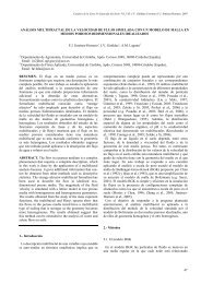
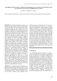
uso <strong>de</strong> <strong>la</strong> ec. (6). La Figura 2 muestra <strong>la</strong> superposición <strong>de</strong><br />
<strong>la</strong>s parejas <strong>de</strong> puntos (t max /t med ,) <strong>con</strong> <strong>la</strong> curva analítica<br />
t max /t med = f () que se obtiene a partir <strong>de</strong> (6), para dos<br />
incrementos <strong>de</strong> humedad distintos =0.05m 3 /m 3 y<br />
=0.5 m 3 /m 3 . Como se pue<strong>de</strong> observar en <strong>la</strong> Figura 2, un<br />
aumento <strong>de</strong> un or<strong>de</strong>n <strong>de</strong> magnitud en <strong>el</strong> incremento <strong>de</strong><br />
humedad,, se traduce en una modificación muy pequeña<br />
en <strong>la</strong> forma <strong>de</strong> <strong>la</strong> curva, lo que explica <strong>la</strong> <strong>de</strong>pen<strong>de</strong>ncia débil<br />
<strong>de</strong> t max /t med = f () <strong>con</strong> , y por tanto <strong>el</strong> que sea<br />
posible representar ésta mediante una única curva<br />
in<strong>de</strong>pendiente <strong>de</strong> Este resultado se discute <strong>con</strong> más<br />
<strong>de</strong>talle en <strong>la</strong> siguiente sección. Evi<strong>de</strong>ntemente, una<br />
expresión analítica <strong>de</strong>l punto t max /t med 5 en <strong>el</strong> que se<br />
alcanzan valores negativos <strong>de</strong> se obtiene <strong>de</strong> t max /t med = f<br />
().<br />
tmax/tmed<br />
(cm)<br />
<br />
max<br />
<br />
0.05 0.1 0.15 0.2 0.25<br />
Fig. 2. Representación <strong>de</strong> los puntos (t max /t med ,) y <strong>la</strong> curva t max /t med = f<br />
() obtenida a partir <strong>de</strong> <strong>la</strong> ec. (6) para dos incrementos <strong>de</strong> humedad<br />
distintos: =0.05m 3 /m 3 (curva inferior) y =0.5 m 3 /m 3 (curva<br />
superior). Nótese que los ejes están invertidos <strong>con</strong> respecto a <strong>la</strong> Figura 1.<br />
3.3. Análisis <strong>de</strong> sensibilidad<br />
De los apartados anteriores queda c<strong>la</strong>ro que <strong>la</strong> re<strong>la</strong>ción<br />
t max /t med juega un pap<strong>el</strong> <strong>de</strong>cisivo en <strong>el</strong> comportamiento <strong>de</strong> K s<br />
y , y por tanto <strong>de</strong> <strong>la</strong> <strong>sortividad</strong> S (2K s ) 1/2 . Es por<br />
<strong>el</strong>lo que dicha re<strong>la</strong>ción t max /t med se utiliza como parámetro <strong>de</strong><br />
variación en <strong>el</strong> análisis <strong>de</strong> sensibilidad que se muestra a<br />
<strong>con</strong>tinuación. Previos trabajos (De Haro et al., 1998) han<br />
obviado <strong>la</strong> importancia <strong>de</strong> <strong>la</strong> re<strong>la</strong>ción t max /t med en <strong>el</strong> análisis<br />
<strong>de</strong> sensibilidad <strong>de</strong> K s . La Figura 3 muestra los coeficientes<br />
<strong>de</strong> sensibilidad (porcentaje <strong>de</strong> variación <strong>con</strong> respecto al<br />
valor inicial) <strong>de</strong> K s , y S para distintas re<strong>la</strong>ciones <strong>de</strong><br />
t max /t med = 2.61, 3.74 y 5.38, haciendo variar o , t max , t med y<br />
en incrementos <strong>de</strong> ±1%, <strong>de</strong>ntro <strong>de</strong>l intervalo [-10%,<br />
10%], alre<strong>de</strong>dor <strong>de</strong>l valor medido. Esto nos permite<br />
investigar <strong>con</strong> qué precisión se <strong>de</strong>ben realizar <strong>la</strong>s medidas<br />
<strong>de</strong> ca<strong>la</strong>do, tiempos máximo y medio así como <strong>de</strong> humedad<br />
<strong>de</strong> <strong>su<strong>el</strong>o</strong>. Nótese que <strong>la</strong>s re<strong>la</strong>ciones t max /t med <strong>el</strong>egidas son<br />
representativas <strong>de</strong> valores <strong>de</strong> K s y lejos o próximos,<br />
respectivamente, <strong>de</strong> <strong>la</strong> región en <strong>la</strong> que pasa a ser<br />
negativa (véase Figura 1). Igualmente se incluye en <strong>el</strong><br />
análisis <strong>de</strong> sensibilidad <strong>el</strong> efecto que tienen sobre <strong>el</strong> valor <strong>de</strong><br />
K s , y S <strong>la</strong>s variaciones en <strong>el</strong> coeficiente 8/ 2 (utilizado<br />
por <strong>Philip</strong> (1993) para ajustar <strong>el</strong> flujo “real” <strong>con</strong> <strong>el</strong> esférico<br />
<strong>de</strong>l mo<strong>de</strong>lo). De esta forma es posible estudiar <strong>la</strong><br />
sensibilidad <strong>de</strong> ésta hipótesis en <strong>la</strong> que está basado <strong>el</strong><br />
mo<strong>de</strong>lo <strong>de</strong> <strong>Philip</strong>. Hay que seña<strong>la</strong>r que este efecto no ha<br />
sido investigado anteriormente.<br />
Varias <strong>con</strong>clusiones pue<strong>de</strong>n obtenerse <strong>de</strong>l análisis <strong>de</strong><br />
sensibilidad presentado en <strong>la</strong> Figura 3: 1) Los tiempos<br />
máximo y medio son los que más influyen en <strong>el</strong> valor final<br />
<strong>de</strong> todas <strong>la</strong>s variables estimadas (K s , y S), pudiendo<br />
compensarse los errores <strong>de</strong> t max y t med , dado que <strong>la</strong>s<br />
perturbaciones que causan en esas variables presentan<br />
signos opuestos (ver también De Haro et al., 1998); 2) La<br />
pendiente <strong>de</strong> <strong>la</strong> curva <strong>de</strong> sensibilidad a t max y t med se invierte<br />
en <strong>el</strong> caso <strong>de</strong> y S <strong>con</strong> respecto al efecto que producen<br />
sobre <strong>la</strong> estimación <strong>de</strong> K s (comparar segunda y tercera fi<strong>la</strong><br />
<strong>de</strong> gráficos <strong>con</strong> <strong>la</strong> primera); 3) La sensibilidad <strong>de</strong> a t max y<br />
t med es mayor que <strong>la</strong> que presentan K s y S, siendo en este<br />
último caso <strong>de</strong>l mismo or<strong>de</strong>n para valores <strong>de</strong> t max /t med bajos<br />
y medios (comparar primera y tercera fi<strong>la</strong> <strong>de</strong> gráficos <strong>con</strong> <strong>la</strong><br />
segunda); 4) La sensibilidad a <strong>la</strong> medida <strong>de</strong> en<br />
cualquiera <strong>de</strong> los casos es insignificante, lo que corrobora<br />
los resultados obtenidos en <strong>la</strong> Figura 2; 5) La sensibilidad al<br />
ca<strong>la</strong>do inicial (h o ) y al coeficiente 8/ 2 es pequeña, sin<br />
embargo es re<strong>la</strong>tivamente importante en <strong>el</strong> caso <strong>de</strong> y S<br />
(no así <strong>de</strong> K s ) para valores <strong>de</strong> t max /t med > 5, próximos al<br />
punto en <strong>el</strong> que pasa a ser negativa; 6) Por último, <strong>la</strong><br />
sensibilidad <strong>de</strong> y S, no así <strong>de</strong> K s , a todos los parámetros<br />
(salvo a aumenta <strong>de</strong> forma drástica a medida que<br />
t max /t med crece, <strong>de</strong> tal manera que en <strong>la</strong> proximidad <strong>de</strong><br />
t max /t med 5, y S se muestran muy sensibles a variaciones<br />
mínimas (< 2%) en los tiempos máximo y medio, <strong>el</strong> ca<strong>la</strong>do<br />
o <strong>el</strong> coeficiente 8/ 2 .<br />
122
Rega<strong>la</strong>do et al. <strong>Medida</strong> <strong>de</strong> <strong>la</strong> Sortividad <strong>de</strong>l Su<strong>el</strong>o <strong>con</strong> <strong>el</strong> permeámetro <strong>de</strong> <strong>Philip</strong>-Dunne<br />
t max /t med =2.61 t max /t med =3.74 t max /t med =5.38<br />
140<br />
120<br />
110<br />
Variación Ks (%)<br />
120<br />
100<br />
80<br />
Variación Ks (%)<br />
110<br />
100<br />
90<br />
Variación Ks (%)<br />
105<br />
100<br />
95<br />
Variación (%)<br />
Variación S (%)<br />
60<br />
200<br />
180<br />
160<br />
140<br />
120<br />
100<br />
80<br />
60<br />
120<br />
110<br />
100<br />
90<br />
-10 -5 0 5 10<br />
Variación Parámetro (%)<br />
-10 -5 0 5 10<br />
Variación Parámetro (%)<br />
-10 -5 0 5 10<br />
Variación Parámetro (%)<br />
Variación (%)<br />
Variación S (%)<br />
80<br />
160<br />
140<br />
120<br />
100<br />
80<br />
60<br />
120<br />
110<br />
100<br />
90<br />
80<br />
-10 -5 0 5 10<br />
Variación Parámetro (%)<br />
-10 -5 0 5 10<br />
Variación Parámetro (%)<br />
-10 -5 0 5 10<br />
Variación Parámetro (%)<br />
Variación (%)<br />
Variación S (%)<br />
90<br />
350<br />
300<br />
250<br />
200<br />
150<br />
100<br />
50<br />
0<br />
280<br />
240<br />
200<br />
160<br />
120<br />
80<br />
40<br />
0<br />
-10 -5 0 5 10<br />
Variación Parámetro (%)<br />
-10 -5 0 5 10<br />
Variación Parámetro (%)<br />
-10 -5 0 5 10<br />
Variación Parámetro (%)<br />
t med t max h <br />
Fig. 3. Análisis <strong>de</strong> sensibilidad <strong>de</strong> K s , y S (eje OY) ante variaciones <strong>de</strong> los parámetros h o , t max , t med , y 8/ 2 (representados por distintos símbolos) en <strong>el</strong><br />
intervalo [-10%, 10%], para distintas re<strong>la</strong>ciones t max /t med = 2.61, 3.74 y 5.38 (<strong>de</strong> izquierda a <strong>de</strong>recha). En <strong>la</strong> última columna <strong>de</strong> gráficos <strong>la</strong>s curvas en <strong>la</strong>s que, a<br />
partir <strong>de</strong> un cierto valor <strong>de</strong> <strong>la</strong> variación en %, <strong>la</strong> pendiente se hace nu<strong>la</strong>, correspon<strong>de</strong>n al valor <strong>de</strong>l parámetro para <strong>el</strong> que < 0 y por tanto <strong>el</strong> algoritmo no<br />
<strong>con</strong>tinua <strong>la</strong> búsqueda <strong>de</strong> soluciones. Nótese que <strong>el</strong> eje OY tiene diferente esca<strong>la</strong> según los gráficos, para así mejorar su visualización.<br />
4. Conclusiones<br />
La medida <strong>de</strong> <strong>la</strong> <strong>sortividad</strong> pue<strong>de</strong> proporcionar<br />
información r<strong>el</strong>evante <strong>de</strong> propieda<strong>de</strong>s hidráulicas y<br />
estructurales <strong>de</strong> un <strong>su<strong>el</strong>o</strong>, como son <strong>la</strong> difusividad, <strong>la</strong><br />
curva <strong>de</strong> <strong>con</strong>ductividad hidráulica y <strong>el</strong> “radio capi<strong>la</strong>r<br />
macroscópico” medio. El permeámetro <strong>de</strong> <strong>Philip</strong>-Dunne<br />
permite estimar <strong>la</strong> <strong>sortividad</strong> a partir <strong>de</strong> mediciones en<br />
campo según S (2K s ) 1/2 . Es por <strong>el</strong>lo que <strong>el</strong> análisis<br />
<strong>de</strong> S, pasa por estudiar <strong>el</strong> comportamiento <strong>de</strong> <strong>la</strong>s<br />
soluciones <strong>de</strong> K s y
Rega<strong>la</strong>do et al. <strong>Medida</strong> <strong>de</strong> <strong>la</strong> Sortividad <strong>de</strong>l Su<strong>el</strong>o <strong>con</strong> <strong>el</strong> permeámetro <strong>de</strong> <strong>Philip</strong>-Dunne<br />
aproximada t max /t med < 5, (estando re<strong>la</strong>cionado este valor<br />
<strong>con</strong> <strong>la</strong>s características <strong>de</strong> diseño, r i y h o , <strong>de</strong>l permeámetro<br />
utilizado) nos permite <strong>de</strong>scartar <strong>el</strong> ensayo en campo, <strong>de</strong><br />
forma rápida, y repetirlo hasta obtener una re<strong>la</strong>ción <strong>de</strong><br />
tiempos apropiada. Por otro <strong>la</strong>do <strong>la</strong> alta sensibilidad <strong>de</strong> <strong>la</strong><br />
<strong>sortividad</strong> y <strong>la</strong> succión en <strong>el</strong> frente <strong>de</strong> avance, en <strong>la</strong> región<br />
próxima a t max /t med 5, sugiere que <strong>la</strong>s medidas <strong>de</strong> tiempos<br />
y ca<strong>la</strong>do <strong>de</strong>ben realizarse <strong>con</strong> gran precisión. Todo <strong>el</strong>lo<br />
refuerza <strong>la</strong> i<strong>de</strong>a <strong>de</strong> <strong>la</strong> necesidad <strong>de</strong> automatización <strong>de</strong> <strong>la</strong>s<br />
lecturas <strong>de</strong> t max /t med y h o , ya explorada por previos autores,<br />
si <strong>el</strong> permeámetro <strong>de</strong> <strong>Philip</strong>-Dunne se preten<strong>de</strong> presentar<br />
como una alternativa sencil<strong>la</strong> a otros métodos para <strong>la</strong><br />
medida <strong>de</strong> <strong>la</strong> <strong>sortividad</strong> en campo.<br />
Con respecto al origen <strong>de</strong> valores <strong>de</strong>