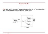
Tema 5: Contraste de hipótesis

Tema 5: Contraste de hipótesis
1
(a partir del material de A. Jach (http://www.est.uc3m.es/ajach/)
y A. Alonso (http://www.est.uc3m.es/amalonso/))
• Conceptos fundamentales: hipótesis nula y alternativa, error de tipo I y
tipo II, función de potencia de un contraste, nivel de significación.
• Contraste de hipótesis e IC.
• Contraste de hipótesis en una población:
• Población normal
• Población no normal pero con muestras de tamaño grande
• Contraste de hipótesis en dos poblaciones independientes:
• Poblaciones normales
• Poblaciones no normales pero con muestras de tamaño grande
• Determinación del tamaño muestral
Estadística I
A. Arribas Gil

2
Definición 1.
Hipótesis estadísticas
Una hipótesis estadística (H) es una proposición acerca de una característica
de la población de estudio. Por ejemplo: “la variable X toma valores en el
intervalo (a, b)”, “el valor de θ es 2”, “la distribución de X es normal”, etc.
Ejemplo 1.
• Una compañía recibe un gran cargamento de piezas. Sólo acepta el envío
si no hay más de un 5% de piezas defectuosas. ¿Cómo tomar una decisión
sin verificar todas las piezas
• Se quiere saber si una propuesta de reforma legislativa es acogida de igual
forma por hombres y mujeres ¿Cómo se puede verificar esa conjetura
Estos ejemplos tienen algo en común:
• Se formula la hipótesis sobre la población.
• Las conclusiones sobre la validez de la hipótesis se basarán en la
información de una muestra.
Estadística I
A. Arribas Gil

Tipos de hipótesis estadísticas
• Hipótesis paramétricas: Una hipótesis paramétrica es una proposición
sobre los valores que toma un parámetro.
3
• Hipótesis simple: aquella que especifica un único valor para el parámetro.
Ejemplos: ‘H : θ = 0”, “H : θ = −23”, etc.
• Hipótesis compuesta: aquella que especifica un intervalo de valores para el
parámetro.
Ejemplos: ‘H : θ ≥ 0”, “H : 1 ≤ θ ≤ 4”, etc.
Hipótesis unilateral: “H : θ ≤ 4”, ‘H : 0 < θ”, etc.
Hipótesis bilateral: “H : θ ≠ 4 ⇔ H : θ < 4 y θ > 4”
• Hipótesis no paramétricas: Una hipótesis no paramétrica es una
proposición sobre cualquier otra característica de la población.
Ejemplos: “H : X ∼ N”, “H : X ind. Y ”, etc. (Tema 6)
Estadística I
A. Arribas Gil

4
Definición 2.
Hipótesis nula y alternativa
Llamamos hipótesis nula, y la representamos por H 0 , a la hipótesis que se
desea contrastar. Es la hipótesis que se plantea en primer lugar y la hipótesis
que mantendremos a no ser que los datos indiquen su falsedad.
Llamamos hipótesis alternativa, y la representamos por H 1 , a la negación de la
hipótesis nula.
Ejemplo 2.
En cursos pasados, el número medio de préstamos por año y por alumno en la
biblioteca de la Carlos III ha sido de 6. Este año la biblioteca ha hecho una
campaña de información y quiere saber el efecto que ésta ha tenido entre los
estudiantes.
¿Cuáles serían las hipótesis nula y alternativa en este caso
Estadística I
A. Arribas Gil

5
Definición 2.
Hipótesis nula y alternativa
Llamamos hipótesis nula, y la representamos por H 0 , a la hipótesis que se
desea contrastar. Es la hipótesis que se plantea en primer lugar y la hipótesis
que mantendremos a no ser que los datos indiquen su falsedad.
Llamamos hipótesis alternativa, y la representamos por H 1 , a la negación de la
hipótesis nula.
Ejemplo 2.
En cursos pasados, el número medio de préstamos por año y por alumno en la
biblioteca de la Carlos III ha sido de 6. Este año la biblioteca ha hecho una
campaña de información y quiere saber el efecto que ésta ha tenido entre los
estudiantes.
¿Cuáles serían las hipótesis nula y alternativa en este caso
H 0 : µ = 6 H 1 : µ > 6
Estadística I
A. Arribas Gil

6
Definición 3.
Contraste de hipótesis
Un contraste de hipótesis es una regla que determina, a un cierto nivel de
significación, α, para qué valores de la muestra se rechaza o no se rechaza la
hipótesis nula.
Es decir, un contraste de hipótesis es una partición del espacio muestral en dos
regiones, una región crítica o de rechazo, RC, y una región de aceptación, RA.
Ω = RC ∪ RA
RC ∩ RA = ∅
Ejemplo 2 (cont.)
Hemos tomado una m.a.s. de 100 alumnos y obtenemos x = 6.23, s = 2.77.
¿Cuál será la región crítica para el contraste H 0 : µ = 6 H 1 : µ > 6
Sea X = “número de libros prestados por alumno y por año”.
E[X ] = µ, Var[X ] = σ 2 ambas desconocidas.
Si H 0 fuera cierta, como n es grande, sabemos que X − 6
S/ √ n
A
∼ N(0, 1).
Estadística I
A. Arribas Gil

Ejemplo 2 (cont.)
Escribiremos
X − 6
S/ √ n
Es decir, si H 0 fuera cierta,
Contraste de hipótesis
A
∼
H 0
N(0, 1).
(
1 − α = P
X −6
S/ √ n < z α
Por tanto, al nivel de significación α,
RC α = {x 1 , . . . , x n | x − 6
s/ √ n > z α} RA α = Ω\RC α = {x 1 , . . . , x n | x − 6
s/ √ n ≤ z α}
Para los datos del ejemplo, n = 100, x = 6.23, s = 2.77, el valor del
estadístico del contraste en nuestra muestra particular es:
x − 6
s/ √ n = 6.23 − 6
2.77/10 = 0.8303
Si consideremos un nivel de significación igual a 0.05, tenemos que
x−6
s/ √ n = 0.8303 < 1.645 = z 0.05, es decir, nuestra muestra particular no
pertenece a la RC 0.05 , y por tanto, al nivel de significación 0.05, no
rechazamos la hipótesis nula.
Estadística I
)
.
7
A. Arribas Gil

Tipos de errores en un contraste de hipótesis
Estado real
8
Decisión H 0 cierta H 0 falsa
Error de Tipo I
Decisión correcta
Rechazar H 0 P(Rech.|H 0cierta) = α P(Rech.|H 0falsa) = 1 − β
nivel de significación
potencia
No rechazar H 0 Decisión correcta Error de Tipo II
P(No Rech.|H 0cierta) = 1 − α P(No Rech.|H 0falsa) = β
1. Podemos hacer la probabilidad del error de tipo I tan pequeña como queramos,
PERO esto hace que aumente la probabilidad del error de tipo II.
2. Un contraste de hipótesis puede rechazar la hipótesis nula pero NO puede
probar la hipótesis nula.
3. Si no rechazamos la hipótesis nula, es porque las observaciones no han aportado
evidencia para descartarla, no porque sea neceseariamente cierta.
4. Por el contrario, si rechazamos la hipótesis nula es porque se está
razonablemente seguro (P(Rech.|H 0cierta) ≤ α) de que H 0 es falsa y estamos
aceptando impĺıcitamente la hipótesis alternativa.
Estadística I
A. Arribas Gil

Definición 4.
Nivel crítico o p-valor
El nivel crítico, p, o p-valor es el nivel de significación más pequeño para el que
la muestra particular obtenida obligaría a rechazar la hipótesis nula. Es decir:
p = P(Rech.H 0 para x 1 , . . . , x n |H 0 cierta)
Es decir, si T (X 1 , . . . , X n ) es el estadístico del contraste:
RC α = {x 1 , . . . , x n | T (x 1 , . . . , x n ) > T α }
RC α = {x 1 , . . . , x n | T (x 1 , . . . , x n ) < T 1−α }
RC α = {x 1 , . . . , x n | |T (x 1 , . . . , x n )| > T α }
=⇒ p = P (T (X 1 , . . . , X n ) > T (x 1 , . . . , x n ))
=⇒ p = P (T (X 1 , . . . , X n ) < T (x 1 , . . . , x n ))
=⇒ p = P (|T (X 1 , . . . , X n )| > |T (x 1 , . . . , x n )|)
9
Estadística I
A. Arribas Gil

Nivel crítico o p-valor
Ejemplo 2 (cont.) Para los datos del ejemplo, n = 100, x = 6.23, s = 2.77,
al nivel de significación 0.05, no rechazamos la hipótesis nula. ¿Cuál es el
p-valor para esta muestra (RC α = {x 1 , . . . , x n | x−6
s/ √ n > z α})
El nivel crítico o p-valor es el nivel de significación más pequeño para el que la
muestra particular obtenida obligaría a rechazar la hipótesis nula:
x 1 , . . . , x n ∈ RC ⇔ x − 6
s/ √ n = z p
⇔ z p = x − 6
s/ √ n = 6.23 − 6
2.77/10 = 0.8303
⇔ p = 0.2033
O equivalentemente,
(
)
X −6
p = P(Rech.|H 0 cierta) = P
S/ √ n > x−6
s/ √ n |H 0cierta
Z= X −6
S/ √ H
∼N(0,1) 0
n
= P(Z > 6.23−6
2.77/10
) = P(Z > 0.8303) = 0.2033
10
Estadística I
A. Arribas Gil

Metodología
11
Método de construcción de un contraste de hipótesis paramétrico al nivel de
significación α:
1. Plantear las hipótesis nula y alternativa (“H 0 : θ = θ 0 , H 1 : θ ≠ θ 0 ”,
“H 0 : θ = θ 0 , H 1 : θ < θ 0 ”,“H 0 : θ ≤ θ 0 , H 1 : θ > θ 0 ”, etc.)
2. Determinar el estadístico del test, T (X 1 , . . . , X n ), y su distribución bajo
H 0 (Formulario).
3. Dos posibilidades:
3.a Construir la región crítica y comprobar si la muestra obtenida está en ella
(rechazamos H 0) o no (no rechazamos H 0).
3.b Calcular el p-valor para la muestra obtenida. Si p < α, se rechaza H 0.
4. Plantear las conclusiones.
Estadística I
A. Arribas Gil

12
Contraste de hipótesis e IC’s
El contraste de una hipótesis nula simple frente a una alternativa bilateral
H 0 : θ = θ 0 H 1 : θ ≠ θ 0
al nivel de significación α, es equivalente a construir un IC al (1 − α)100%
para θ, y a partir de él tomar la siguiente decisión:
• rechazar H 0 si θ 0 está fuera del IC.
• no rechazar H 0 si θ 0 está en el IC.
Es decir IC (1−α)100% (θ) = RA α .
Ejemplo 3.
Supongamos que la altura (en cm) de los estudiantes de la UC3M es una v.a.
X con distribución N(µ, 5). Con el objetivo de estimar µ se toma una m.a.s.
de 100 estudiantes y se obtiene x = 156.8. (Ejemplo 1 Tema 4)
Se quiere contrastar la siguiente hipótesis sobre esta población: “la altura
media de los estudiantes de la UC3M es de 160cm” al nivel de significación
0.05.
Estadística I
A. Arribas Gil

13
Contraste de hipótesis e IC’s
Ejemplo 3 (cont.)
Seguimos los pasos de la metodología para la construcción de contrastes:
1. Plantear las hipótesis nula y alternativa:
H 0 : µ = 160 H 1 : µ ≠ 160
2. Determinar el estadístico del test y su distribución bajo H 0 (Formulario).
X ∼ N(µ, 5), por tanto
X − µ
5/ √ n
∼ N(0, 1) ⇒
X − 160
5/ √ n
H 0
∼ N(0, 1)
Estadística I
A. Arribas Gil

Contraste de hipótesis e IC’s
Ejemplo 3 (cont.)
14
3.a Construir la región crítica y comprobar si la muestra obtenida está en ella
(rechazamos H 0 ) o no (no rechazamos H 0 ). Sabemos que bajo H 0
Por tanto
RC α =
(
1 − α = P −z α < X − 160 )
2
5/ √ n < z α
2
{
x 1 , . . . , x n |
RA α = Ω\RC α =
∣
∣ x−160
5/ √ n
∣ > z α
2
{
x 1 , . . . , x n |
Recordemos que el IC al (1 − α)100% para µ era
160 ∈IC ⇔ x−z α
2
5
√ n
≤ 160 ≤ x+z α
2
∣
}
∣ x−160
5/ √ n
5
√ n
⇔ |x−160| ≤ z α
2
∣ ≤ z α
2
(
x ± z α
2
}
5 √ n
):
5
√ n
⇔ x 1 , . . . , x n ∈RA α
Estadística I
A. Arribas Gil

Contraste de hipótesis e IC’s
15
Ejemplo 3 (cont.)
Para α = 0.05 (n = 100, x = 156.8):
∣ x − 160
∣ 5/ √ ∣∣∣ n ∣ = 156.8 − 160
5/10 ∣ = |−3.2| = 3.2 y z α = 1.96
2
es decir x 1 , . . . , x n ∈ RC 0.05 ⇒ rechazamos H 0 al nivel de significación 0.05.
O equivalentemente, a partir del IC al 95% para µ:
( ) (
5
x ± z α √ = 156.8 ± 1.96 5 )
= (155.82, 157.78)
2 n 10
160 /∈ IC 95% (µ) ⇒ rechazamos H 0 al nivel de significación 0.05.
Hemos comprobado que es equivalente realizar el contraste al 0.05% a
encontrar el IC para µ al 95% y rechazar H 0 si µ 0 no está en él.
Estadística I
A. Arribas Gil

Ejemplo 3 (cont.)
Contraste de hipótesis e IC’s
16
3.b (Otra alternativa) Calcular el p-valor para la muestra obtenida.
p = P(Rech.H 0 para x 1 , . . . , x n |H 0 cierta)
(∣ )
∣∣ X −160
= P
5/ √ n
∣ > ∣ x−160
5/ √ n
∣ |H 0 cierta
Z= X −160
5/ √ H
∼N(0,1) 0 (
)
n
= P |Z| > ∣ 156.8−160
∣ = P(|Z| > 6.4) = 2 · P(Z > 6.4) ≈ 0
5/10
El p-valor obtenido es menor que α (p ≈ 0

17
Contraste de hipótesis en una población
Sea X una v.a. cuya distribución depende de θ. X 1 , . . . , X n m.a.s. de X .
Sea T (X 1 , . . . , X n ) el estadístico del contraste }
T (X 1 , . . . , X n ) H0
∼ P 0
y T α el cuantil α de P 0 .
Formulario ∗
H 0 H 1 RC α
θ = θ 0 θ ≠ θ 0
{
x1 . . . , x n | |T (X 1 , . . . , X n )| > T α/2
}
θ ≤ θ 0 θ > θ 0 {x 1 . . . , x n | T (X 1 , . . . , X n ) > T α }
θ ≥ θ 0 θ < θ 0 {x 1 . . . , x n | T (X 1 , . . . , X n ) < T 1−α ∗∗ }
∗ Como siempre, dos casos posibles: X normal o X no normal pero n grande (TCL).
Hay que formular siempre TODAS las hipótesis necesarias.
∗∗ Si P 0 es simétrica (normal o t-student), entonces T 1−α=−T α.
Estadística I
A. Arribas Gil

Contraste de hipótesis en dos poblaciones independientes
Sea X una v.a. cuya distribución depende de θ 1 . X 1 , . . . , X n1 m.a.s. de X .
Sea Y una v.a. cuya distribución depende de θ 2 . Y 1 , . . . , Y n2 m.a.s. de Y .
X e Y independientes.
Sea T (X 1:n1 , Y 1:n2 ) el estadístico del contraste
}
T (X 1:n1 , Y 1:n2 ) H0
∼ P 0
y T α el cuantil α de la distribución de P 0 .
Formulario ∗
18
H 0 H 1 RC α
θ 1 − θ 2 = d ∗∗
0 θ 1 − θ 2 ≠ d 0
{
x1:n1 , y 1:n2 | |T (X 1 , . . . , X n )| > T α/2
}
θ 1 − θ 2 ≤ d 0 θ 1 − θ 2 > d 0 {x 1:n1 , y 1:n2 | T (X 1 , . . . , X n ) > T α }
θ 1 − θ 2 ≥ d 0 θ 1 − θ 2 < d 0 {x 1:n1 , y 1:n2 | T (X 1 , . . . , X n ) < T 1−α }
∗ Como siempre, dos casos posibles: X , Y normales o X , Y no normales pero n
grande (TCL). Hay que formular siempre TODAS las hipótesis necesarias.
∗∗ En general, en la comparación de varianzas d 0 = 0.
Estadística I
A. Arribas Gil

Definición 5.
Determinación del tamaño muestral
La potencia o función potencia del contraste paramétrico
19
H 0 : θ ∈ Θ 0 H 1 : θ ∈ Θ 1 = Θ\Θ 0
se define como
p(θ 1 ) = 1 − β(θ 1 ) = 1 − P(Error de Tipo II) = P(Rech. H 0 | H 0 falsa)
= P(Rech. H 0 | θ = θ 1 ), ∀θ 1 ∈ Θ 1 .
Ejemplo 3 (cont.)
Para el contraste
teníamos
RC α =
H 0 : µ = 160 H 1 : µ ≠ 160
{
x 1 , . . . , x n |
∣
x − 160
5/ √ n
∣ > z α
2
}
.
Estadística I
A. Arribas Gil

Ejemplo 3 (cont.)
Determinación del tamaño muestral
La función de potencia de este contraste es:
20
p(µ 1 ) = P(Rech. H 0 | µ = µ 1 ) = P
( X − 160
= P
(∣ ∣∣∣ X − 160
5/ √ n
)
∣ > z α | µ = µ
2 1
5/ √ n < −z α
2
o X − 160
5/ √ n > z α
2
| µ = µ 1
)
(
= P X < 160 − z α
2
( X − µ1
[tipif.] = P
[
Z=
X −µ 1
5/ √ n
]
µ=µ
∼ 1
N(0,1)
= P
5/ √ n < 160 − µ 1
5/ √ n
5
√ n
o X > 160 + z α
2
)
5
√ | µ = µ 1 n
− z α o X − µ 1
2
5/ √ n > 160 − µ 1
5/ √ n
+ z α
2
| µ = µ 1
)
(
Z < 160 − µ 1
5/ √ − z α o Z > 160 − µ )
1
2
n
5/ √ + z α , ∀µ
2
1 ≠ 160.
n
Estadística I
A. Arribas Gil

Determinación del tamaño muestral
21
Ejemplo 3 (cont.)
¿Cómo es p(µ 1 ) en función de n
¿Y en función de |µ 0 − µ 1 |
Dada σ y prefijado el nivel de significación, el objetivo es obtener una potencia
mayor o igual que un cierto valor (valores usuales 0.9 ó 0.8) cuando la
diferencia entre la media verdadera, µ 1 , y la hipotética, µ 0 , supere un valor
prefijado.
Buscaremos el tamaño de muestra mínimo que verifique esa condición.
Estadística I
A. Arribas Gil