1.5. Integral de lÃnea de un campo Vectorial.
1.5. Integral de lÃnea de un campo Vectorial.
1.5. Integral de lÃnea de un campo Vectorial.

You also want an ePaper? Increase the reach of your titles
YUMPU automatically turns print PDFs into web optimized ePapers that Google loves.
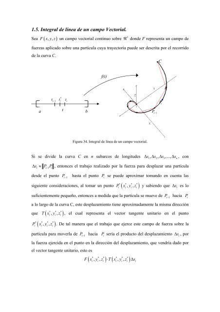
<strong>1.5.</strong> <strong>Integral</strong> <strong>de</strong> línea <strong>de</strong> <strong>un</strong> <strong>campo</strong> <strong>Vectorial</strong>.Sea F ( xyz , , ) <strong>un</strong> <strong>campo</strong> vectorial continuo sobre3R don<strong>de</strong> F representa <strong>un</strong> <strong>campo</strong> <strong>de</strong>fuerzas aplicado sobre <strong>un</strong>a partícula cuya trayectoria pue<strong>de</strong> ser <strong>de</strong>scrita por el recorrido<strong>de</strong> la curva C.Cf(t)Piati− 1*ti ti*PitbPi− 1Figura 34. <strong>Integral</strong> <strong>de</strong> línea <strong>de</strong> <strong>un</strong> <strong>campo</strong> vectorial.Si se divi<strong>de</strong> la curva C en n subarcos <strong>de</strong> longitu<strong>de</strong>s ∆s 1, ∆s 2, ∆s 3,..., ∆ sn, con∆s≈ P P , entonces el trabajo realizado por la fuerza para <strong>de</strong>splazar <strong>un</strong>a partículai i−1i<strong>de</strong>s<strong>de</strong> el p<strong>un</strong>to Pi− 1hasta el p<strong>un</strong>to P ise pue<strong>de</strong> aproximar tomando en cuenta las* * * *siguiente consi<strong>de</strong>raciones, al tomar <strong>un</strong> p<strong>un</strong>toi ( i, i,i )P x y z y sabiendo que ∆ sies losuficientemente pequeño, entonces a medida que la partícula se mueve <strong>de</strong> Pi− 1haciaa lo largo <strong>de</strong> la curva C, este <strong>de</strong>splazamiento tiene aproximadamente la misma dirección* * *que ( i, i,i )T x y z , el cual representa el vector tangente <strong>un</strong>itario en el p<strong>un</strong>to( , , )P x y z . De tal manera que el trabajo que ejerce este <strong>campo</strong> <strong>de</strong> fuerza sobre la* * * *i i i ipartícula para moverla <strong>de</strong> Pi− 1haciaPisería el producto <strong>de</strong>l <strong>de</strong>splazamientoPi∆ si, porla fuerza ejercida en el p<strong>un</strong>to en la dirección <strong>de</strong>l <strong>de</strong>splazamiento, que vendría dado porel vector tangente <strong>un</strong>itario, esto es* * * * * *( , , ) ⋅ ( , , )F x y z T x y z ∆ si i i i i i i
por tanto el trabajo total que ejerce el <strong>campo</strong> <strong>de</strong> fuerza para <strong>de</strong>splazar la partícula <strong>de</strong>s<strong>de</strong>su p<strong>un</strong>to inicial hasta el p<strong>un</strong>to final vendría dado, en forma aproximada, por laexpresiónn∑i=1( * , * , * ) ⋅ ( * , * ,*)F x y z T x y z ∆si i i i i i iPara tener <strong>un</strong>a aproximación más cercana al valor verda<strong>de</strong>ro <strong>de</strong>l trabajo total realizadose pue<strong>de</strong> incrementar el número <strong>de</strong> subarcos n en el que se ha dividido la curva C. Alestudiar el límite <strong>de</strong> estas aproximaciones se obtiene el valor exacto <strong>de</strong>l trabajo totalrealizado es:n→∞ i = 1n∑ ( * * * ) ( * * *i, i, i i, i, i ) i ∫ ( , , ) ( , , )W = Lim F x y z ⋅T x y z ∆ s = F x y z ⋅T x y z dsConsi<strong>de</strong>rando que la curva C tiene como parametrización a la f<strong>un</strong>ción vectorial3R→R () = ( () () ( )), el vector tangente <strong>un</strong>itario ( )g: / g t x t , y t , z t()T t() t() t= g'g', <strong>de</strong> manera que la ecuación anterior se podría reescribir como() t() tCT t viene dado porb⎡g'⎤bW = ∫ ⎢F( x() t , y() t , z()t ) ⋅ ⎥ g' () t dt = F( x() t , y() t , z()t ) g'() t dtag'∫ a⎢⎣⎥⎦Ahora bien esta interpretación ha sido <strong>de</strong>sarrollada para el caso en que el <strong>campo</strong>vectorial es <strong>un</strong> <strong>campo</strong> <strong>de</strong> fuerza, sin embargo po<strong>de</strong>mos basarnos en este <strong>de</strong>sarrollo para<strong>de</strong>finir al integral <strong>de</strong> línea <strong>de</strong> <strong>un</strong> <strong>campo</strong> vectorial <strong>de</strong> la manera que se presenta acontinuaciónDefinición. Sea F <strong>un</strong> <strong>campo</strong> vectorial <strong>de</strong>finido por( ) ( 1( ) 2( ) 3( ))3 3F: D / F X F X , F X , F X⊆R →R = , y sea C <strong>un</strong>a curva, <strong>de</strong>finida en D,3dada paramétricamente por la f<strong>un</strong>ción vectorial g: R→R / g( t) = ( x( t) , y( t) , z( t))con t∈[ a,b], entonces la integral <strong>de</strong> línea <strong>de</strong>l <strong>campo</strong> vectorial F sobre C es igual a∫ ∫ ∫C C ab( ()) '()F⋅ dr = F⋅ Tdl = F g t ⋅g t dt
∫ ∫ ∫ ∫ ∫CF ⋅ dr = F ⋅ dr + F ⋅ dr + F ⋅ dr + F ⋅drC1 C2 C3 C4∫C ∫1 C ∫2 C ∫3 C42 3 2 3∫ x dy ( 2 ) ( 2 )C ∫ y xy dx1 C ∫ x dy y xy dx2 C ∫3 C4−−∫ ()() ∫ () () ∫ ∫= F dx + F dy + F dx + F dy + F dx + F dy + F dx + F dy1 2 1 2 1 2 1 2= + + + + +( )() ( )() (() ())()1 2 1 3 1 2 1 3−1 1 1 −1= 1 1 dt + 1 + 2t 1 1 dt + − 1 1 dt + 1 + 2t 1 1 dt= 0EJERCICIOS PROPUESTOS <strong>1.5.</strong>1.1) Evalúe cada <strong>un</strong>a <strong>de</strong> las siguientes integrales <strong>de</strong> línea∫Cyzdx + xzdy + xydz, don<strong>de</strong> Cestá formada por los segmentos rectilíneos que <strong>un</strong>en al p<strong>un</strong>to ( 1, 0, 0 ) con ( 0,1,0 ) y aéste con ( 0,0,1 ).2x22) Sea F( x, y, z) ( xe ,3x y)= . Determine la integral <strong>de</strong> F a lo largo <strong>de</strong>l perímetro <strong>de</strong>lrectángulo con vértices en los p<strong>un</strong>tos ( 0,0 ) , ( 3, 0 ) ( 3, 2 ) y ( 0, 2 ) , recorrido en sentidopositivo.<strong>1.5.</strong>2. Significado físico <strong>de</strong> la integral <strong>de</strong> línea <strong>de</strong> <strong>un</strong> <strong>campo</strong> vectorial F.Otra interpretación física <strong>de</strong> la integral <strong>de</strong> línea es cuando la f<strong>un</strong>ción vectorial V es<strong>campo</strong> <strong>de</strong> velocida<strong>de</strong>s <strong>de</strong> <strong>un</strong> fluido, el significado que tiene la integral <strong>de</strong> línea∫ V ⋅Tdr es la cantidad <strong>de</strong> fluido circula a lo largo <strong>de</strong> la curva C por <strong>un</strong>idad <strong>de</strong> tiempo,Cen la dirección <strong>de</strong>l vector tangente <strong>un</strong>itario T, si la curva C es <strong>un</strong>a curva cerrada, laintegral <strong>de</strong> F sobre esta curva se escribe∫ V ⋅T dr y se le <strong>de</strong>nomina como la integralC<strong>de</strong> circulación <strong>de</strong> V alre<strong>de</strong>dor d la curva C. Si la f<strong>un</strong>ción V representa <strong>un</strong> <strong>campo</strong> <strong>de</strong>velocida<strong>de</strong>s <strong>de</strong> <strong>un</strong> fluido, la integral <strong>de</strong> línea∫ V ⋅ Ndr se interpreta como el flujo queCatraviesa a la región acotada por la curva C por <strong>un</strong>idad <strong>de</strong> tiempo, en la dirección <strong>de</strong>lvector <strong>un</strong>itario N, y a se le <strong>de</strong>nomina como integral <strong>de</strong> flujo <strong>de</strong> V a través <strong>de</strong> C.En el caso que <strong>un</strong> <strong>campo</strong> vectorial continuo B represente <strong>un</strong> <strong>campo</strong> magnético, laintegral <strong>de</strong> línea∫ B ⋅ Ndr representa la cantidad <strong>de</strong> corriente que atraviesa la regiónCR acotada por la curva C, mientras que si la f<strong>un</strong>ción vectorial E es <strong>un</strong> <strong>campo</strong> eléctrico
continuo sobre alg<strong>un</strong>a región R, entonces la integral <strong>de</strong> línea <strong>de</strong>∫CB ⋅ Ndr, se interpretacomo el flujo <strong>de</strong>l <strong>campo</strong> eléctrico a través <strong>de</strong> la región R.EJEMPLO 32. Sobre <strong>un</strong>a partícula en el plano se aplica <strong>un</strong> <strong>campo</strong> <strong>de</strong> fuerza dado por2y( , ) ( ,2 )F x y = y + y xy− e , la trayectoria <strong>de</strong> dicha partícula se <strong>de</strong>scribe por el arco enel primer cuadrante <strong>de</strong> la circ<strong>un</strong>ferencia x2 + y2 = 1, y luego por la recta x + y = 1,siguiendo el sentido <strong>de</strong> las agujas <strong>de</strong>l reloj. Determine el trabajo que ejerce el <strong>campo</strong> <strong>de</strong>fuerzas sobre la partícula a través <strong>de</strong> la trayectoria <strong>de</strong>scrita.Figura 37. Trayectoria recorrida por la partícula <strong>de</strong>l Ejemplo 32.Solución. La parametrización <strong>de</strong> la curva que <strong>de</strong>scribe la trayectoria <strong>de</strong> la partículaviene dado por C C1 C222[ ] ( ) ( )= ∪ , don<strong>de</strong> C : 0, 2 / g( θ ) ( cos θ,senθ)1⎡ π ⎤⎢ →R =⎣ 2 ⎥⎦C :0,1 →R / g t = t ,1− t , la integral <strong>de</strong> línea para <strong>de</strong>terminar el trabajo ejercidosobre dicha partícula viene planteada pory
∫C( , )W = F x y ⋅dr∫( , ) ( , )= F x y ⋅ dr+ F x y ⋅dr∫C1 C2∫( , ) ( , ) ( , ) ( , )= F x y dx+ F x y dy+ F x y dx+F x y dy1 2 1 2C1 C2∫πdd2= ∫ F1( x( θ) , y( θ)) ( x( θ)) d( θ) + F2( x( θ) , y( θ)) ( y( θ)) d( θ)0dθdθ0dd+ ∫ F1( x() t , y()t ) ( x()t ) d() t + F2( x() t , y()t ) ( y()t ) d()t1dtdtπ2 2sen( θ )= ⎡( sen ( θ ) sen( θ))( sen( θ)) ( 2cos( θ) sen( θ)e )( cos( θ)) ⎤∫ + − + −d ( θ)0 ⎣⎦02+ ⎡( ( 1− t) + ( 1− t))() 1 + ( 2t( 1−t))( 1) ⎤∫− d( t)1 ⎣⎦π2 3 2 2sen( θ⎡)sen ( ) sen ( ) 2cos ( ) sen( ) e cos d0 ⎣⎦0 2 2∫∫( 1 t) ( 1 t) 2t 2t ⎤d( t)( ) ⎤ ( )= − θ − θ + θ θ − θ θ+ ⎡ − + − − +1 ⎣⎦π3 23 3 sen2 3⎡ 1 2 2 ⎤=⎢cos( θ) − cos ( θ) − cos ( θ)− e + ⎢− − − t + t ⎥⎣ 3 3 ⎥⎦ 3 2 30 ⎢⎣⎥⎦⎡ 1 1 2⎤= [ 1− e]+⎢− − + 1−⎣ 3 2 3⎥⎦1= −e22( θ ) ⎤ ⎡ ( 1−t) ( 1−t)EJEMPLO 33. La fuerza en <strong>un</strong> p<strong>un</strong>to ( x, yz , ) esta dada por F ( xyz , , ) ( yzx , , )01= .Calcule el trabajo realizado por F( x, y,z ) sobre <strong>un</strong>a partícula que <strong>de</strong>scribe latrayectoria dada por la curva C:0,2 [ ] →R 3 / f ( t) = ( t, t 2 , t3)
Figura 38. Trayectoria recorrida por la partícula <strong>de</strong>l Ejemplo 33.Solución. El trabajo realizado por la fuerza F viene dado por la integral <strong>de</strong> línea∫CF⋅dr, como ya se conoce la parametrización <strong>de</strong> la curva C, que <strong>de</strong>scribe la trayectoria<strong>de</strong> la partícula, se obtiene2( , , )W = F x y z ⋅dr( , , ) ( , , ) ( , , )1 2 3() 1 ( 2 ) ( 3 )= ⎡0 ⎣+ +2= ∫⎡0 ⎣ + + ⎤⎦⎡1 3 2 5 3 4⎤=⎢t + t + t⎣3 5 4 ⎥⎦8 64= + + 123 5412=15EJERCICIOS PROPUESTOS <strong>1.5.</strong>3.∫C∫= F xyzdx+ F xyzdy+F xyzdzC∫= ydx + zdy + xdz1) La fuerza en <strong>un</strong> p<strong>un</strong>to ( , )C∫2 3 2t t t t t dt2 4 3t 2t 3t dttrabajo realizado por F( x, y,z ) sobre la curvap<strong>un</strong>to ( 2,8 ).20⎤⎦x y esta dada por F( x, y) ( x 2 y 2 , xy)y= + . Determine el3= x <strong>de</strong>s<strong>de</strong> el p<strong>un</strong>to ( )0,0 hasta el
2) La fuerza en <strong>un</strong> p<strong>un</strong>to ( , , )x yz esta dada por F( x, y, z) ( e x , e y , ez)= . Calcule eltrabajo realizado por F( x, y,z ) sobre <strong>un</strong>a partícula que <strong>de</strong>scribe la trayectoria dada porla curva C:0,2 [ ] →R 3 / f () t = ( t, t 2 , t3)3) Si el trabajo realizado por el <strong>campo</strong> <strong>de</strong> fuerzas F( x, y, z) ( 3 xy, 5 z 2 , x)= − para mover<strong>un</strong>a partícula a lo largo <strong>de</strong> la curva C, dada paramétricamente por3 2 2C:0, [ t0] →R / f ( t) = ( t + 1, t , t)es 1543t0.<strong>un</strong>ida<strong>de</strong>s <strong>de</strong> trabajo, <strong>de</strong>termine el valor <strong>de</strong><strong>1.5.</strong>4. Velocidad tangencial promedio <strong>de</strong> <strong>un</strong> fluido.Si <strong>un</strong>a f<strong>un</strong>ción V ( x, y,z ) representa <strong>un</strong> <strong>campo</strong> <strong>de</strong> velocida<strong>de</strong>s <strong>de</strong> <strong>un</strong> fluido en3R laintegral <strong>de</strong> línea∫CV ⋅ dr, don<strong>de</strong> C es <strong>un</strong>a curva suave o parcialmente suave, cerrada yrecorrida en forma positiva, se pue<strong>de</strong> interpretar como la cantidad neta <strong>de</strong> giro <strong>de</strong>lfluido en el sentido <strong>de</strong> recorrido <strong>de</strong> la curva C. Se pue<strong>de</strong> aquí observar lo siguiente: si∫ V ⋅ dr > 0 entonces las partículas <strong>de</strong>l fluido se <strong>de</strong>splazan en el sentido <strong>de</strong> recorrido <strong>de</strong>C∫la curva; si por el contrario V ⋅ dr < 0 , entonces las partículas <strong>de</strong>l fluido se <strong>de</strong>splazanCen el sentido contrario al <strong>de</strong>l recorrido <strong>de</strong> la curva C y si el <strong>campo</strong> vectorial V es∫perpendicular a la curva C, entonces V ⋅ dr = 0 , en este caso el fluido se dice que esirrotacional.CAhora bien, también es posible <strong>de</strong>terminar la velocidad tangencial promedio <strong>de</strong> <strong>un</strong>fluido sobre la curva cerrada C, o circulación promedio <strong>de</strong>l <strong>campo</strong> V sobre la curva Cmediante la siguiente integral1V = V ⋅TdrS∫CEn don<strong>de</strong> S representa la superficie <strong>de</strong> la región que está acotada por la curva cerrada C.
EJEMPLO 34. Si la velocidad <strong>de</strong> <strong>un</strong> fluido está <strong>de</strong>scrita por V ( x, y) ( yx,y)C= .Determine la circulación <strong>de</strong> F a lo largo <strong>de</strong> la curva C, sabiendo que la curva C es lacirc<strong>un</strong>ferencia con centro en el origen coor<strong>de</strong>nadas y con radio 2.Solución. La circulación <strong>de</strong> V a lo largo <strong>de</strong> la curva C, viene dado por la integral <strong>de</strong>línea ∫ V ⋅Tdr, la curva C se pue<strong>de</strong> parametrizar como() ( ) [ ]2g: / g t 2cos t,2 sent , t 0,2πR→R = ∈ , como ya se conoce la parametrización <strong>de</strong>la curva C, que <strong>de</strong>scribe la trayectoria <strong>de</strong> la partícula, se calcula la integral <strong>de</strong> línea <strong>de</strong> lasiguiente manera:∫CCC2π02π0( , )W = V x y ⋅dr∫( , ) ( , )= V x y dx+V x y dy∫1 2= yxdx + ydy∫( 2 )( 2cos )( 2s ) ( 2 )( 2cos )= ⎡⎣sent t − ent + sent t ⎤⎦dt∫2= ⎡⎣− 8sen t cost + 4sent cost⎤⎦dt⎡ 8 3 2 ⎤=⎢− sen t + 2sen t⎣ 3⎥⎦= 0El <strong>campo</strong> F no realiza trabajo sobre la partícula.2π0EJEMPLO 35. Si la velocidad <strong>de</strong> <strong>un</strong> fluido está <strong>de</strong>scrita por2( , , ) ( ,2 , )V x y z = x xy+ x z . Determine la circulación <strong>de</strong> V a lo largo <strong>de</strong> la curva C,sabiendo que la curva C es la circ<strong>un</strong>ferencia <strong>un</strong>itaria con centro en el origen <strong>de</strong>coor<strong>de</strong>nadas, en el plano z = 0 .Solución. La curva C pue<strong>de</strong> ser parametrizada por la expresión vectorial() ( ) [ ]3g: / g t cos t, sent,0 , t 0,2πR→R = ∈ , la integral <strong>de</strong> línea para calcular lacirculación <strong>de</strong>l fluido se <strong>de</strong>fine <strong>de</strong> la siguiente manera:
∫CCC( , , )W = V x y z ⋅dr∫( , , ) ( , , ) ( , , )= V xyzdx+ V xyzdy+V xyzdz∫1 2 3( 2 )= + + +∫2xdx xy x dy zdz( cos ) ( s ) ( 2 cos cos )( cos ) ( 0)( 0)2π2= ⎡ t − ent + sent t + t t + ⎤ dt0 ⎣⎦∫2π0() () cos ()2 2= ⎡⎣cost sen t + t ⎤⎦dt⎡ 1 3 1 1 ⎤=⎢− cos t+ t+sen( 2t)⎣ 3 2 4 ⎥⎦= πEl fluido circula en el sentido contrario al <strong>de</strong> las agujas <strong>de</strong>l reloj.2π0EJERCICIOS PROPUESTOS <strong>1.5.</strong>4.1) Si la velocidad <strong>de</strong> <strong>un</strong> fluido está <strong>de</strong>scrita por F( x, y, z) ( x 2 ,2 xy x,z)= + . Determinela circulación <strong>de</strong> F a lo largo <strong>de</strong> la curva C, sabiendo que la curva C es la circ<strong>un</strong>ferenciacon centro en el origen <strong>de</strong> coor<strong>de</strong>nadas y radio 1, en el plano z = 0 .2) Si la velocidad <strong>de</strong> <strong>un</strong> fluido está <strong>de</strong>scrita por F( x, y, z) ( x 2 ,2 xy x,z)= + . Determinela circulación <strong>de</strong> F a lo largo <strong>de</strong> la curva C, sabiendo que la curva C es la circ<strong>un</strong>ferenciacon centro en el origen <strong>de</strong> coor<strong>de</strong>nadas y radio 1, en el plano z = 0 .