representacion-de-senales-en-wolfram-mathematica (1)

Laboratorio #1
Nombre : Hugo Paul Rengifo Carrión
Paralelo : "B"
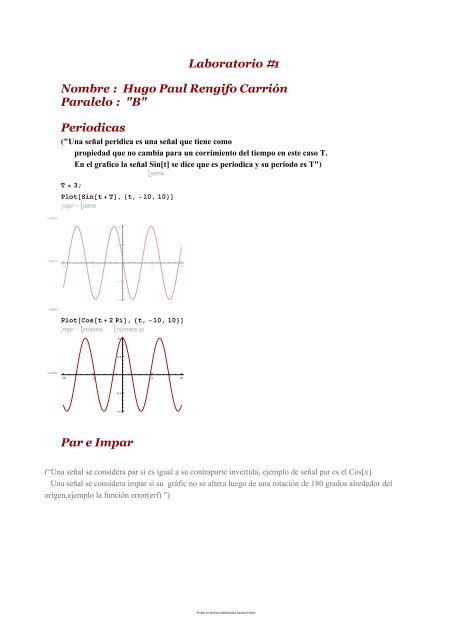
Periodicas
("Una señal peridica es una señal que tiene como
propiedad que no cambia para un corrimiento del tiempo en este caso T.
En el grafico la señal Sin[t] se dice que es periodica y su periodo es T")
T = 3;
seno
Plot[ Sin[t + T], {t, -10, 10}]
repr⋯ seno
Out[85]=
1.0
0.5
Out[87]=
-10 -5 5 10
-0.5
-1.0
In[98]:=
Plot[ Cos[t + 2 Pi], {t, -10, 10}]
repr⋯ coseno número pi
1.0
0.5
Out[98]=
-10 -5 5 10
-0.5
-1.0
Par e Impar
(“Una señal se considera par si es igual a su contraparte invertida, ejemplo de señal par es el Cos[x]
Una señal se considera impar si su gráfic no se altera luego de una rotación de 180 grados alrededor del
origen,ejemplo la función error(erf) ”)
Printed by Wolfram Mathematica Student Edition

2 Lab1.nb
In[100]:=
Plot[{-Erf[x],
Erf[-x]}, {x, -10, 10}]
represe⋯ función e⋯función error
1.0
0.5
Out[100]=
-10 -5 5 10
-0.5
-1.0
In[39]:=
Plot[{ Cos[x], Cos[-x]}, {x, -10, 10}]
repre⋯ coseno coseno
1.0
0.5
Out[39]=
-10 -5 5 10
-0.5
-1.0
Exponenciales y Senoidales
(“Son funciones las cuales dependiendo del tiempo su amplitud se ve aumentada, estas
señales son la base fundamental para crear otras señales mas complejas”)
Plot[ Exp[x], {x, -5, 5}]
repr⋯ exponencial
60
50
40
30
20
10
-4 -2 2 4
Printed by Wolfram Mathematica Student Edition

Lab1.nb 3
Plot[ Exp[-x], {x, -5, 5}]
repr⋯ exponencial
60
50
40
30
20
10
-4 -2 2 4
Plot[ Sin[4 x], {x, -5, 5}]
repr⋯ seno
1.0
0.5
-4 -2 2 4
-0.5
-1.0
Plot[ Sin[x / 2], {x, -10, 10}]
repr⋯ seno
1.0
0.5
-10 -5 5 10
-0.5
-1.0
DiscretePlot[
representación discreta
{1.09^n Cos[(2 Pi n) / 15] + 1.09^n Sin[(2 Pi n) / 15], 1.1^n, -1.1^n}, {n, 0, 50}]
coseno número pi
seno número pi
100
50
10 20 30 40 50
-50
Printed by Wolfram Mathematica Student Edition

4 Lab1.nb
DiscretePlot[
representación discreta
{0.94^n Cos[(2 Pi n) / 18] + 0.94^n Sin[(2 Pi n) / 18], 0.94^n, -0.94^n}, {n, 0, 50}]
coseno número pi
seno número pi
1.0
0.5
10 20 30 40 50
-0.5
-1.0
Impulso unitario y Escalón unitario
("Una funcion escalon unitario tiene como caracteristica principal que tiene un valor de 0 para todos
los valores negativos de su argumento y de 1 para todos los valores positivos de su argumento
Una funcion, el impulso unitario vale 1 solo en el argumento y para todos los demas valores toma valor de 0")
DiscretePlot[ DiscreteDelta[n], {n, -2, 2}, PlotTheme → "Business"]
representación d⋯ delta discreta
tema de representación
1.0
0.8
0.6
0.4
0.2
0
-2 -1 0 1 2
DiscretePlot[ DiscreteDelta[n - 2], {n, -2, 2}, PlotTheme → "Business"]
representación d⋯ delta discreta
tema de representación
1.0
0.8
0.6
0.4
0.2
0
-2 -1 0 1 2
Printed by Wolfram Mathematica Student Edition

Lab1.nb 5
Plot[ UnitStep[x], {x, -5, 5}]
repr⋯ función paso unidad
1.0
0.8
0.6
0.4
0.2
-4 -2 2 4
Plot[ UnitStep[x - 3], {x, -5, 5}]
repr⋯ función paso unidad
1.0
0.8
0.6
0.4
0.2
-4 -2 2 4
Sumatoria de convolucion
(“La convolución de señales en una manera muy general de realizar un promediomóvil
y para nuestro caso, convolucionando una señal ruidosa con un filtro respuesta de
impulso de duración finita (FIR), obtenemos una señal muy suavizada y filtrada.
Para obtener la salida y[n] en un cierto instante fijo n, primero se dibujan h[k] y la versión
“abatida y desplazada” x[n-k] sobre el eje k. En segundo lugar, se multiplican
ambas señales para obtener la señal h[k] x[n-k]. Si se suman todos los valores de la
nueva señal con respecto a k obtendremos el valor de y[n]. ”)
Printed by Wolfram Mathematica Student Edition

6 Lab1.nb
In[78]:=
h = (2)^n UnitStep[-n];
función paso unidad
Z =
UnitStep[n];
función paso unidad
DiscreteConvolve[h, Z, n, m]
convolución discreta
DiscretePlot[%, {m, -10, 10}]
representación discreta
Out[80]= 2 m ≥ 0
2 1+m True
2.0
1.5
Out[81]=
1.0
0.5
-10 -5 5 10
Integral de convolución
In[40]:= h = Exp[-2 x] UnitStep[x];
exponencial función paso unidad
Out[41]=
Convolve[h, UnitStep[x], x, y]
convoluciona función paso unidad
Plot[%, {y, 0, 10}, PlotRange → All]
representación gráfica rango de repr⋯ todo
e -y Sinh[y] UnitStep[y]
0.5
0.4
0.3
Out[42]=
0.2
0.1
2 4 6 8 10
Printed by Wolfram Mathematica Student Edition