TP microcontrôleur 16 bits : filtrage de signaux ... - J.-M Friedt
TP microcontrôleur 16 bits : filtrage de signaux ... - J.-M Friedt
TP microcontrôleur 16 bits : filtrage de signaux ... - J.-M Friedt

You also want an ePaper? Increase the reach of your titles
YUMPU automatically turns print PDFs into web optimized ePapers that Google loves.
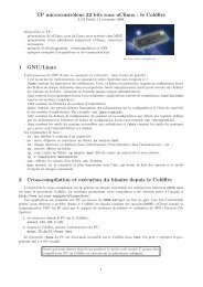
<strong>TP</strong> <strong>microcontrôleur</strong> <strong>16</strong> <strong>bits</strong> : <strong>filtrage</strong> <strong>de</strong> <strong>signaux</strong> numériques<br />
J.-M <strong>Friedt</strong>, 17 novembre 2009<br />
Objectif <strong>de</strong> ce <strong>TP</strong> :<br />
– exploiter les fonctions <strong>de</strong> traitement du signal <strong>de</strong> GNU/Octave pour concevoir un filtre<br />
– implémenter ce filtre dans un <strong>microcontrôleur</strong> <strong>16</strong> <strong>bits</strong><br />
– vali<strong>de</strong>r expérimentalement le fonctionnement du filtre<br />
1 Conception d’un filtre <strong>de</strong> réponse finie (FIR)<br />
Le sujet <strong>de</strong> ce <strong>TP</strong> n’est pas <strong>de</strong> développer la théorie <strong>de</strong>s filtres numériques mais uniquement <strong>de</strong> rappeler quelques uns <strong>de</strong>s<br />
concepts utiles en pratique :<br />
– un filtre <strong>de</strong> réponse impulsionnelle finie [1] (Finite Impulse Response, FIR) bm est caractérisé par une sortie yn à un<br />
instant donné n qui ne dépend que <strong>de</strong>s valeurs actuelle et passées <strong>de</strong> la mesure xm, m ≤ n :<br />
yn = <br />
k=0..m<br />
bkxn−k<br />
L’application du filtre s’obtient pas convolution <strong>de</strong>s coefficients du filtre et <strong>de</strong>s mesures.<br />
– un filtre <strong>de</strong> réponse impulsionnelle infinie (IIR) a une sortie qui dépend non seulement <strong>de</strong>s mesures mais aussi <strong>de</strong>s<br />
valeurs passées du filtre.<br />
– GNU/Octave (et Matlab) proposent <strong>de</strong>s outils <strong>de</strong> synthèse <strong>de</strong>s filtres FIR et IIR. Par soucis <strong>de</strong> stabilité numérique et<br />
simplicité d’implémentation, nous ne nous intéresserons qu’aux FIR. Dans ce cas, les coefficient <strong>de</strong> récursion sur les<br />
valeurs passées du filtre (nommées en général am dans la littérature) seront égaux à a = 1.<br />
Le calcul d’un filtre dont la réponse spectrale ressemble à une forme imposée par l’utilisateur (suivant un critère <strong>de</strong>s<br />
moindres carrés) est obtenu par la fonction firls(). Cette fonction prend en argument l’ordre du filtre (nombre <strong>de</strong> coefficients),<br />
la liste <strong>de</strong>s fréquences définissant le gabarit du filtre et les magnitu<strong>de</strong>s associées. Elle renvoie la liste <strong>de</strong>s coefficients<br />
b.<br />
L’application d’un FIR <strong>de</strong> coefficients b (avec a=1) ou <strong>de</strong> façon plus générale d’un IIR <strong>de</strong> coefficients a et b sur un vecteur<br />
<strong>de</strong> données expérimentales x s’obtient par filter(b,a,x) ;<br />
Tout filtre se définit en terme <strong>de</strong> fréquence normalisée : la fréquence 1 correspond à la <strong>de</strong>mi-fréquence d’échantillonnage<br />
(fréquence <strong>de</strong> Nyquist) lors <strong>de</strong> la mesure <strong>de</strong>s données.<br />
Exercices :<br />
1. en supposant que nous échantillonnons les données sur un convertisseur analogique-numérique à <strong>16</strong>000 Hz, i<strong>de</strong>ntifier<br />
les coefficients d’un filtre passe-ban<strong>de</strong> entre 700 et 900 Hz. Combien faut-il <strong>de</strong> coefficients pour obtenir un résultat<br />
satisfaisant ?<br />
2. Quelle est la conséquence <strong>de</strong> choisir trop <strong>de</strong> coefficients ? Quelle est la conséquence <strong>de</strong> choisir trop peu <strong>de</strong> coefficients ?<br />
3. ayant obtenu la réponse impulsionnelle du filtre, quelle est sa réponse spectrale ?<br />
4. vali<strong>de</strong>r sur <strong>de</strong>s données (boucle sur les fréquences) simulées la réponse spectrale du filtre<br />
Au lieu <strong>de</strong> boucler sur <strong>de</strong>s fréquences et observer la réponse du filtre appliqué à un signal monochromatique, le chirp est<br />
un signal dont la fréquence instantanée évolue avec le temps. Ainsi, la fonction<br />
chirp([0 :1/<strong>16</strong>000 :5],40,5,8000) ;<br />
génère un signal échantillonné à <strong>16</strong> kHz, pendant 5 secon<strong>de</strong>s, balayant la gamme <strong>de</strong> fréquences allant <strong>de</strong> 40 Hz à 8 kHz.<br />
Exercices :<br />
1. appliquer le filtre i<strong>de</strong>ntifié auparavant au chirp, et visualiser le signal issu <strong>de</strong> cette transformation<br />
2. que se passe-t-il si la fréquence <strong>de</strong> fin du chirp dépasse 8 kHz dans cet exemple ?<br />
2 Application pratique du filtre<br />
Exercices : Implémenter sur MSP430<br />
1. sachant que les acquisitions se font sur 12 <strong>bits</strong>, quelle est la plage <strong>de</strong> valeur sur laquelle se font les mesures ?<br />
2. comment exploiter les coefficients numériques du filtre pour un calcul sur <strong>de</strong>s entiers sur <strong>16</strong> <strong>bits</strong> (short) ? sur 32 <strong>bits</strong><br />
(long) ?<br />
1. l’échantillonnage périodique <strong>de</strong> mesures analogiques acquises sur ADC0<br />
2. l’affichage du résultat <strong>de</strong> ces mesures<br />
3. le <strong>filtrage</strong> <strong>de</strong> ces mesures par un FIR synthétisé selon la métho<strong>de</strong> vue plus haut<br />
4. l’affichage du résultat <strong>de</strong> ce <strong>filtrage</strong><br />
5. l’affichage <strong>de</strong> l’amplitu<strong>de</strong> du signal résultant du <strong>filtrage</strong><br />
6. appliquer ce programme à une mesure sur un chirp généré par la carte son du PC au moyen <strong>de</strong> audacity<br />
1
7. comparer l’expérience et la simulation.<br />
Exemple <strong>de</strong> programme et résultats :<br />
#i n c l u d e <br />
#i n c l u d e <br />
#i n c l u d e <br />
#i n c l u d e <br />
#i n c l u d e <br />
#un<strong>de</strong>f <strong>de</strong>bug<br />
void Sommeil ( void ) ;<br />
void Pause TIMERB( unsigned s h o r t Compteur ) ;<br />
void Pause ms ( unsigned s h o r t ms) ;<br />
i n t e r r u p t (TIMERB0 VECTOR ) wakeup Vector TIMERB0 ( void ) ;<br />
void i n i t h o r l o g e ( void ) ;<br />
void init PORT ( void ) ;<br />
void init TIMER ( void ) ;<br />
void i n i t r s 1 9 6 0 0 ( ) {<br />
UCTL1=SWRST; // SetupUART1 : mov . b #SWRST,&UCTL1 ; c f p.13 −4<br />
UCTL1|=CHAR; // b i s . b #CHAR,&UCTL1<br />
UTCTL1=SSEL0 ; // mov . b #SSEL0,&UTCTL1 ; 32768 Hz ACLK<br />
UBR01=0x03 ; // mov . b #0x03 ,&UBR01 ; 4800 bauds<br />
UBR11=0x00 ; // mov . b #0x00 ,&UBR11<br />
UMCTL1=0x4A ; // mov . b #0x4A,&UMCTL1<br />
UCTL1&=˜SWRST; // b i c . b #SWRST,&UCTL1<br />
ME2|=UTXE1+URXE1; // b i s . b #UTXE1+URXE1,&ME2<br />
}<br />
void s n d r s 1 ( unsigned char cara )<br />
{ w h i l e ( ( IFG2 & UTXIFG1)==0) ; // j z r s t x 1<br />
TXBUF1=cara ;<br />
}<br />
void s t r r s 1 ( unsigned char ∗ cara )<br />
{ i n t k=0;<br />
do { s n d r s 1 ( cara [ k ] ) ; k++;} w h i l e ( cara [ k ] ! = 0 ) ;<br />
}<br />
void init PORT ( void ) {<br />
P1SEL = 0 x00 ;<br />
P1DIR = 0xFF ;<br />
P1OUT = 0 x00 ;<br />
}<br />
P3SEL=0xFE ; // mov . b #0xF0,&P3SEL ; P3 . 6 , 7 = USART s e l e c t<br />
P3DIR=0x5B ; // mov . b #0x50 ,&P3DIR ; P3 . 6 = output d i r e c t i o n<br />
P3OUT=0x01 ; // mov . b #0x00 ,&P3OUT ; P3 . 6 = output v a l<br />
void init ADC ( void ) {<br />
ADC12CTL0=SHT0 6+REFON+ADC12ON; // V REF=1.5 V<br />
ADC12CTL1=SHP; // mov .w #SHP,&ADC12CTL1<br />
ADC12MCTL0=INCH 0+SREF 1 ; // mov . b #INCH 10+SREF 1 &ADC12MCTL0<br />
ADC12CTL0|=ENC; // b i s .w #ENC,&ADC12CTL0<br />
}<br />
unsigned s h o r t temperature ( )<br />
{ADC12CTL0|=ADC12SC ; // s t a r t c o n v e r s i o n<br />
do {} w h i l e ( (ADC12CTL1 & 1) !=0) ;<br />
r e t u r n (ADC12MEM0) ;<br />
}<br />
i n t e r r u p t (TIMERA0 VECTOR ) wakeup Vector TIMERA0 ( void )<br />
{ }<br />
void i n i t h o r l o g e ( void ) {<br />
BCSCTL1 = 0 x87 ;<br />
BCSCTL2 = SELM1 + SELS ;<br />
WDTCTL = WD<strong>TP</strong>W + WDTHOLD;<br />
}<br />
long f i l t r e ( unsigned s h o r t ∗ in , long ∗ f i l , long nin , long n f i l , long ∗ s o r t i e )<br />
{ unsigned s h o r t k , j ; long s =0,max=−2500;<br />
i f ( nin>n f i l )<br />
{ f o r ( k=0;k
}<br />
s o r t i e [ k]= s ;<br />
i f (max
#e n d i f<br />
s p r i n t f ( chaine ,”%% %l d \ r \n ” ,max) ;<br />
s t r r s 1 ( c h a i n e ) ;<br />
}<br />
e l s e {P1OUT=0x00 ; }<br />
}<br />
r e t u r n ( 0 ) ;<br />
}<br />
magntitu<strong>de</strong> (u.a.)<br />
magnitu<strong>de</strong> (u.a.)<br />
800<br />
600<br />
400<br />
200<br />
0<br />
-200<br />
-400<br />
1<br />
0.5<br />
0<br />
-0.5<br />
-1<br />
0 500 1000 1500 2000 2500 3000 3500 4000<br />
frequence (Hz)<br />
firls(<strong>16</strong>0,[0 600 700 900 1000 fe/2]/fe*2,[0 0 1 1 0 0]);<br />
0 500 1000 1500 2000 2500 3000 3500 4000<br />
magnitu<strong>de</strong> (u.a.)<br />
fe=<strong>16</strong>000;<br />
ffin=4000;<br />
f<strong>de</strong>b=40;<br />
b=firls(<strong>16</strong>0,[0 600 700 900 1000 fe/2]/fe*2,[0 0 1 1 0 0]);<br />
x=chirp([0:1/fe:5],f<strong>de</strong>b,5,ffin);<br />
f=linspace(f<strong>de</strong>b,ffin,length(x));<br />
plot(f,filter(b,1,x));<br />
freq=[f<strong>de</strong>b:150:ffin];<br />
k=1;<br />
for f=freq<br />
x=sin(2*pi*f*[0:1/fe:1]);<br />
y=filter(b,1,x);<br />
sortie(k)=max(y);<br />
k=k+1;<br />
end<br />
hold on;plot(freq,sortie,’r’)<br />
xlabel(’frequence (Hz)’)<br />
ylabel(’magnitu<strong>de</strong> (u.a.)’)<br />
3 Conception d’un filtre <strong>de</strong> réponse infinie (IIR)<br />
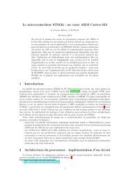
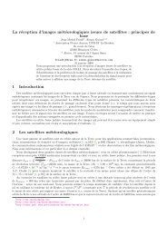
En haut à gauche : mesure expérimentale <strong>de</strong> la réponse d’un FIR passe<br />
ban<strong>de</strong> conçu pour être passant entre 700 et 900 Hz. La mesure est effectuée<br />
au moyen d’un chirp <strong>de</strong> 40 à 4000 Hz en 30 secon<strong>de</strong>s généré par une carte<br />
son d’ordinateur. En bas à gauche : modélisation <strong>de</strong> la réponse d’un filtre<br />
passe ban<strong>de</strong> entre 700 et 900 Hz, en bleu par <strong>filtrage</strong> d’un chirp, en rouge<br />
par calcul <strong>de</strong> l’effet du filtre sur quelques <strong>signaux</strong> monochromatiques. Ci-<br />
<strong>de</strong>ssus : programme GNU/Octave <strong>de</strong> la simulation.<br />
GNU/Octave propose les fonctions cheb et butter pour concevoir <strong>de</strong>s filtres IIR. Une fois les coefficients b et a (cette<br />
fois a est un vecteur) l’IIR se tient compte non seulement <strong>de</strong>s <strong>de</strong>rnières observations mais aussi <strong>de</strong>s valeurs passées du filtre :<br />
yn = <br />
bkxn−k − <br />
k=0..m<br />
k=1..m<br />
akyn−k<br />
Exercice :<br />
Exploiter ces fonctions pour concevoir un filtre aux performances comparables aux IIR proposés ci-<strong>de</strong>ssus, et implémenter<br />
ces filtres dans le MSP430 pour en vali<strong>de</strong>r le fonctionnement.<br />
4 Expression explicite dans le domaine fréquentiel<br />
L’efficacité <strong>de</strong>s filtres vus auparavant est leur application dans le domaine temporel : une fois les coefficients a et b<br />
i<strong>de</strong>ntifiés, l’application du filtre consiste en N multiplication pour un filtre d’ordre N.<br />
Le passage dans le domaine fréquentiel par transformée <strong>de</strong> Fourier nécessite un calcul considérablement plus long. L’approche<br />
naïve <strong>de</strong> la transformée <strong>de</strong> Fourier nécessite N multiplications, puisque chacun <strong>de</strong>s N termes en sortie nécessite<br />
lui-même N multiplications<br />
Xn = <br />
xk exp (−2iπk × n/N)<br />
k=0..N−1<br />
L’exploitation <strong>de</strong> la transformée <strong>de</strong> Fourier rapi<strong>de</strong> (FFT) exploite les symétries <strong>de</strong> la formule vue ci-<strong>de</strong>ssus pour utiliser<br />
autant <strong>de</strong> fois que nécessaire les mêmes termes xk exp (−2πk × n/N) qui apparaissent plusieurs fois : on notera [2, p.432] la<br />
4
elation suivante entre les termes pairs F p n et les termes impairs F i n <strong>de</strong> la transformée <strong>de</strong> Fourier Fn<br />
=<br />
<br />
k=0..N/2−1<br />
=<br />
<br />
m=0..M−1<br />
Xn = <br />
k=0..N−1<br />
x2k exp (2iπ2k × n/N) +<br />
x2m exp (2iπm × n/N) +<br />
xk exp (2iπk × n/N)<br />
<br />
k=0..N/2−1<br />
<br />
m=0..M−1<br />
= Pn + exp(−2iπn/N)In<br />
x2k+1 exp (2iπ(2k + 1) × n/N)<br />
x2m+1 exp (2iπm × n/N)<br />
en posant M = N/2, et avec Pn le calcul sur les indices pairs et In le calcul sur les indices impairs. Chaque calcul d’un terme<br />
<strong>de</strong> FFT nécessite donc N opérations, mais ceci le long d’un arbre binaire <strong>de</strong> longueur log 2(N) au lieu <strong>de</strong> N. La complexité<br />
du calcul est donc passée <strong>de</strong> N 2 à N log 2(N).<br />
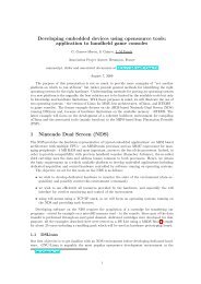
L’implémentation <strong>de</strong> cet algorithme est décrit en détail dans la note d’application 3722 <strong>de</strong> Maxim 1 .<br />
frequence (FFT sur 256 points<br />
max(|FFT|)<br />
120<br />
100<br />
80<br />
60<br />
40<br />
20<br />
440 Hz, 880 Hz, chirp 440-1320 Hz en 30 secon<strong>de</strong>s<br />
0<br />
0 100 200 300 400 500 600 700<br />
9000<br />
8000<br />
7000<br />
6000<br />
5000<br />
4000<br />
3000<br />
2000<br />
1000<br />
0<br />
0 100 200 300 400 500 600 700<br />
temps (u.a.)<br />
indice fréquence<br />
(point) (Hz)<br />
11 440<br />
21 880<br />
31 1320<br />
On a bien le point 256 qui correspond<br />
à la fréquence 10900 qui est<br />
égale à 32768/3.<br />
La principale optimisation reste ensuite l’exploitation du<br />
multiplieur matériel disponible dans le MSP430. L’étu<strong>de</strong><br />
du co<strong>de</strong> assembleur généré par msp430-gcc -S démontre<br />
que le compilateur est capable <strong>de</strong> convertir le symbole * en<br />
la séquence d’opérations exploitant au mieux le matériel.<br />
Un autre aspect intéressant <strong>de</strong> l’étu<strong>de</strong> du co<strong>de</strong> <strong>de</strong> la note d’application AN3722 est <strong>de</strong> constater la génération automatique<br />
<strong>de</strong> co<strong>de</strong> pour précalculer un certain nombre <strong>de</strong> constantes. Ainsi, la réorganisation <strong>de</strong>s données pour passer <strong>de</strong> la transformée<br />
<strong>de</strong> Fourier classique à la FFT est générée automatiquement, ainsi que les tables contenant les fonctions trigonométriques<br />
pré-calculées. Par ailleurs, cette génération <strong>de</strong> co<strong>de</strong> automatique est très sensible à la nature <strong>de</strong>s données manipulées. Les<br />
casts successifs (long sur 4 octets et short sur 2 octets) sont nécessaires pour le bon fonctionnement <strong>de</strong> ce co<strong>de</strong> :<br />
resultMulReCos=((long)cosLUT[tf_in<strong>de</strong>x]*(long)x_n_re[b_in<strong>de</strong>x])>>7;<br />
resultMulReSin=((long)sinLUT[tf_in<strong>de</strong>x]*(long)x_n_re[b_in<strong>de</strong>x])>>7;<br />
resultMulImCos=((long)cosLUT[tf_in<strong>de</strong>x]*(long)x_n_im[b_in<strong>de</strong>x])>>7;<br />
1 http://www.maxim-ic.com/appnotes.cfm/an pk/3722<br />
5
esultMulImSin=((long)sinLUT[tf_in<strong>de</strong>x]*(long)x_n_im[b_in<strong>de</strong>x])>>7;<br />
x_n_re[b_in<strong>de</strong>x] = x_n_re[a_in<strong>de</strong>x]-(short)resultMulReCos+(short)resultMulImSin;<br />
x_n_im[b_in<strong>de</strong>x] = x_n_im[a_in<strong>de</strong>x]-(short)resultMulReSin-(short)resultMulImCos;<br />
x_n_re[a_in<strong>de</strong>x] = x_n_re[a_in<strong>de</strong>x]+(short)resultMulReCos-(short)resultMulImSin;<br />
x_n_im[a_in<strong>de</strong>x] = x_n_im[a_in<strong>de</strong>x]+(short)resultMulReSin+(short)resultMulImCos;<br />
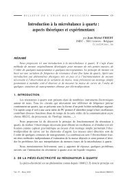
frequence (Hz)<br />
0<br />
1000<br />
2000<br />
3000<br />
4000<br />
5000<br />
imagesc([1 232],[2*10900/256 10900/2],minicom’)<br />
0 50 100 150 200<br />
temps (u.a.)<br />
Spectrogramme obtenu par émission d’un signal à 440 Hz, puis 880 Hz, puis un chirp et finalement les <strong>de</strong>ux fréquences<br />
initiales générées simultanément.<br />
#i n c l u d e <br />
#i n c l u d e <br />
#i n c l u d e <br />
#i n c l u d e ” maxqfft . h”<br />
#d e f i n e msp430<br />
#i f d e f msp430<br />
#i n c l u d e <br />
#i n c l u d e <br />
#i n c l u d e <br />
#i n c l u d e <br />
#e n d i f<br />
// msp430−gcc −mmcu=msp430x149 −c msp430 . c<br />
// msp430−gcc −mmcu=msp430x149 −o maxqfft msp430 . o maxqfft . c<br />
// s i n o n gcc −o maxqfft maxqfft . c −lm<br />
s h o r t x n r e [ N f f t ] ; // FFT input samples , and r e a l part o f the spectrum<br />
void getSamplesFromADC ( )<br />
{ unsigned s h o r t i ;<br />
s h o r t ∗ p t r x n r e = x n r e ;<br />
f o r ( i =0; i
{<br />
#i f d e f msp430<br />
unsigned char b u f f e r [ 2 0 ] ;<br />
init PORT ( ) ;<br />
init ADC ( ) ;<br />
i n i t r s 1 9 6 0 0 ( ) ;<br />
init TIMER ( ) ;<br />
e i n t ( ) ;<br />
TACTL|= MC 1 + TACLR;<br />
#e n d i f<br />
#i f d e f msp430<br />
w h i l e ( 1 ) // FFT Loop<br />
#e n d i f<br />
{<br />
unsigned s h o r t i ; // Misc in<strong>de</strong>x<br />
s h o r t n o f b = N DIV 2 ; // Number o f b u t t e r f l i e s<br />
s h o r t s o f b = 1 ; // S i z e o f b u t t e r f l i e s<br />
s h o r t a i n d e x = 0 ; // f f t data in<strong>de</strong>x<br />
s h o r t a i n d e x r e f = 0 ; // f f t data in<strong>de</strong>x r e f e r e n c e<br />
char s t a g e = 0 ; // Stage o f the f f t , 0 to ( Log2 (N) −1)<br />
s h o r t nb in<strong>de</strong>x ; // Number o f b u t t e r f l i e s in<strong>de</strong>x<br />
s h o r t s b i n d e x ; // S i z e o f b u t t e r f l i e s in<strong>de</strong>x<br />
s h o r t x n im [ N f f t ] = {0 x0000 } ; // Imaginary part o f x ( n ) and X( n ) ,<br />
bzero ( x n r e , s i z e o f ( s h o r t ) ∗ N f f t ) ;<br />
bzero ( x n im , s i z e o f ( s h o r t ) ∗ N f f t ) ;<br />
getSamplesFromADC ( ) ;<br />
/∗ Perform Bit−R e v e r s a l : Uses an u n r o l l e d loop that was c r e a t e d<br />
with the f o l l o w i n g C co<strong>de</strong> :<br />
∗/<br />
#i n c l u d e <br />
#d e f i n e N 256<br />
#d e f i n e LOG 2 N 8<br />
s h o r t bitRev ( s h o r t a , s h o r t nBits )<br />
{ s h o r t r e v a = 0 ;<br />
f o r ( s h o r t i =0; i >7;<br />
resultMulImCos =(( long ) cosLUT [ t f i n d e x ] ∗ ( long ) x n im [ b in<strong>de</strong>x ] ) >>7;<br />
7
}<br />
resultMulImSin =(( long ) sinLUT [ t f i n d e x ] ∗ ( long ) x n im [ b in<strong>de</strong>x ] ) >>7;<br />
x n r e [ b in<strong>de</strong>x ] = x n r e [ a i n d e x ] −( s h o r t ) ( resultMulReCos+resultMulImSin ) ;<br />
x n im [ b in<strong>de</strong>x ] = x n im [ a i n d e x ] −( s h o r t ) ( resultMulReSin−resultMulImCos ) ;<br />
x n r e [ a i n d e x ] = x n r e [ a i n d e x ]+( s h o r t ) ( resultMulReCos−resultMulImSin ) ;<br />
x n im [ a i n d e x ] = x n im [ a i n d e x ]+( s h o r t ) ( resultMulReSin+resultMulImCos ) ;<br />
i f ( ( ( s b i n d e x +1) & ( s o f b −1) ) == 0)<br />
a i n d e x = a i n d e x r e f ;<br />
e l s e<br />
a i n d e x++;<br />
t f i n d e x += n o f b ;<br />
}<br />
a i n d e x = ( ( s o f b = 1 ;<br />
s o f b
{<br />
+128 ,+127 ,+127 ,+127 ,+127 ,+127 ,+126 ,+126 ,+125 ,+124 ,+124 ,+123 ,+122 ,+121 ,+120 ,+119 ,<br />
+118 ,+117 ,+115 ,+114 ,+112 ,+111 ,+109 ,+108 ,+106 ,+104 ,+102 ,+100 , +98, +96, +94, +92,<br />
+90, +88, +85, +83, +81, +78, +76, +73, +71, +68, +65, +63, +60, +57, +54, +51,<br />
+48, +46, +43, +40, +37, +34, +31, +28, +24, +21, +18, +15, +12, +9, +6, +3,<br />
+0, −3, −6, −9, −12, −15, −18, −21, −24, −28, −31, −34, −37, −40, −43, −46,<br />
−48, −51, −54, −57, −60, −63, −65, −68, −71, −73, −76, −78, −81, −83, −85, −88,<br />
−90, −92, −94, −96, −98 , −100 , −102 , −104 , −106 , −108 , −109 , −111 , −112 , −114 , −115 , −117 ,<br />
−118 , −119 , −120 , −121 , −122 , −123 , −124 , −124 , −125 , −126 , −126 , −127 , −127 , −127 , −127 , −127<br />
} ;<br />
/∗<br />
s i n e Look−Up Table : An LUT f o r the s i n e f u n c t i o n<br />
c r e a t e d with the f o l l o w i n g program :<br />
#i n c l u d e <br />
#i n c l u d e <br />
#d e f i n e N 256<br />
void<br />
{<br />
main ( i n t argc , char ∗ argv [ ] )<br />
p r i n t f (” c o n s t long sinLUT[%d ] =\n{\n ” ,N/2) ;<br />
f o r ( long<br />
{<br />
i =0; i
}<br />
P3SEL=0xFE ; // ; P3 . 6 , 7 = USART s e l e c t<br />
P3DIR=0x5B ; // ; P3 . 6 = output d i r e c t i o n<br />
P3OUT=0x01 ; // ; P3 . 6 = output v a l<br />
void init ADC ( void ) {<br />
ADC12CTL0=SHT0 6+REFON+ADC12ON; // V REF=1.5 V<br />
ADC12CTL1=SHP;<br />
ADC12MCTL0=INCH 0+SREF 1 ; // p .17 −11: s i n g l e c o n v e r s i o n<br />
ADC12CTL0|=ENC;<br />
}<br />
unsigned s h o r t mesure ( )<br />
{ADC12CTL0|=ADC12SC ; // s t a r t c o n v e r s i o n<br />
do {} w h i l e ( (ADC12CTL1 & 1) !=0) ;<br />
r e t u r n (ADC12MEM0) ;<br />
}<br />
void init TIMER ( void ) {<br />
BCSCTL1 = 0 x87 ; // XT2 OFF<br />
BCSCTL2 = SELM1 + SELS ; // LFXT2 : use HF quartz (XT2) i f a v a i l a b l e<br />
WDTCTL = WD<strong>TP</strong>W + WDTHOLD; // Stop WDT<br />
TACTL=TASSEL0 + TACLR;<br />
TACCTL0|=CCIE ; // CCR0 i n t e r r u p t enabled<br />
TACCR0=2;<br />
TACTL|= MC 0 ;<br />
}<br />
i n t e r r u p t (TIMERA0 VECTOR ) wakeup Vector TIMERA0 ( void )<br />
{ }<br />
Listing 3 – Quelques fonctions pour la communication et initialisation du MSP430<br />
Lors du traitement <strong>de</strong> N données réelles, nous exploitons <strong>de</strong>s tableaux <strong>de</strong> N éléments réels et N éléments imaginaires<br />
(2N cases mémoire) pour n’exploiter à la fin que N/2 éléments <strong>de</strong> la transformée <strong>de</strong> Fourier Xn puisque XN−n = X ∗ n. Il est<br />
possible d’optimiser l’occupation mémoire en plaçant la moitié <strong>de</strong>s données initiales dans le tableau <strong>de</strong> la partie imaginaire <strong>de</strong>s<br />
donnés en entrée : alors l’intégralité <strong>de</strong> la transformée <strong>de</strong> Fourier est exploitée, et les relations <strong>de</strong> symétrie entre transformée<br />
<strong>de</strong> données purement réelles (XN−n = X ∗ n) et purement imaginaires (XN−n = −X ∗ n) permettent d’i<strong>de</strong>ntifier quelle partie <strong>de</strong><br />
la transformée <strong>de</strong> Fourier vient <strong>de</strong> quelle donnée initiale.<br />
Pour s’en convaincre, sous GNU/Octave :<br />
c l e a r<br />
c l o s e<br />
x=s i n (2∗ p i ∗ [ 0 : 0 . 0 1 : 1 0 . 2 3 ] ∗ 3 )+i ∗ 0 ;<br />
f 1=f f t ( x ( 1 : 5 1 2 ) ) ; % 512 complexes<br />
f 2=f f t ( x ( 5 1 3 : 1 0 2 4 ) ) ; % 512 complexes<br />
xx=x ( 1 : 5 1 2 )+i ∗x ( 5 1 3 : 1 0 2 4 ) ; % 256 v a l s<br />
f f=f f t ( xx ) ; % 256 complexes<br />
re1 ( 1 )=r e a l ( f f ( 1 ) ) ;<br />
re2 ( 1 )=imag ( f f ( 1 ) ) ;<br />
f o r j j =1:255<br />
re1 ( j j +1)=r e a l ( 0 . 5 ∗ ( f f ( j j +1)+f f (512− j j +1) ) ) ;<br />
im1 ( j j +1)=imag ( 0 . 5 ∗ ( f f ( j j +1)− f f (512− j j +1) ) ) ;<br />
re2 ( j j +1)=imag ( 0 . 5 ∗ ( f f ( j j +1)+f f (512− j j +1) ) ) ;<br />
im2 ( j j +1)=−r e a l ( 0 . 5 ∗ ( f f ( j j +1)− f f (512− j j +1) ) ) ;<br />
end<br />
p l o t ( r e a l ( f 1 ( 1 : 2 5 6 )−re1 ) )<br />
hold on<br />
p l o t ( imag ( f 1 ( 1 : 2 5 6 ) )−im1 , ’ g ’ )<br />
p l o t ( r e a l ( f 2 ( 1 : 2 5 6 ) )−re2 , ’ r ’ )<br />
p l o t ( imag ( f 2 ( 1 : 2 5 6 ) )−im2 , ’m’ )<br />
Listing 4 – Comparaison entre le résultat d’une FFT sur N points, et le résultat du calcul exploitant les parties réelles et<br />
imaginaires d’un tableau <strong>de</strong> N/2 points.<br />
Références<br />
[1] A.V. Oppenheim & R.W. Schafer, Discrete-Time Signal Processing, Prentice Hall (1989)<br />
[2] W.H. Press, B.P. Flannery, S.A. Teukolsky, & W.T. Vertterling, Numerical recipies in Pascal, Cambridge University Press (1994), ou sur le<br />
web http://en.wikipedia.org/wiki/Cooley%E2%80%93Tukey FFT algorithm<br />
10