Correction TD 1 analyse de données Exercice 1:

ESA 3 TD1 analyse de données: correction p. 1
Correction TD 1 analyse de données I-3-c
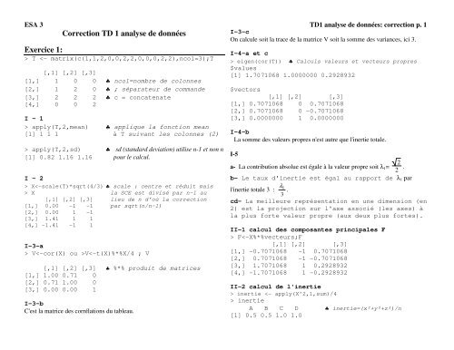
On calcule soit la trace de la matrice V soit la somme des variances, ici 3.
Exercice 1:
> T apply(T,2,mean) ♣ applique la fonction mean
[1] 1 1 1 à T suivant les colonnes (2)
> apply(T,2,sd) ♣ sd (standard deviation) utilise n-1 et non n
[1] 0.82 1.16 1.16 pour le calcul.
I - 2
> X X la SCE est divisé par n-1 au
[,1] [,2] [,3] lieu de n d'où la correction
[1,] 0.00 -1 -1 par sqrt(n/n-1)
[2,] 0.00 1 -1
[3,] 1.41 1 1
[4,] -1.41 -1 1
I-3-a
> VV F

ESA 3 TD1 analyse de données: correction p. 2
II-3 calcul des QLT
III-1 Calcul des coordonnées des variables G
> G diag(inertie^(-1))%*%F^2/4
[,1] [,2] [,3]
[1,] 0.25 0.50 0.25 ♣ diag : matrice
[2,] 0.25 0.50 0.25 diagonale des
[3,] 0.73 0.25 0.02 inverses des inerties
[4,] 0.73 0.25 0.02
II-4 calcul des CTR
> F^2%*%diag(eigen(V)$values^(-1))/4
[,1] [,2] [,3]
[1,] 0.07 0.25 0.43 ♣ diag(eigen(V)$values^(-1))
[2,] 0.07 0.25 0.43 matrice diagonale avec
[3,] 0.43 0.25 0.07 l'inverse des valeurs propres.
[4,] 0.43 0.25 0.07
II-5
> plot(F[,1],F[,2],main="plan F1 F2")
Individus
♣ plot(x,y) : nuage de points avec x=F1 y=F2
III-2 CTR des variables
>vecteurs%*%G^2%*%diag(eigen(cor(X))$values^(-1)
[,1] [,2] [,3]
[1,] 0.5 0 0.5
[2,] 0.5 0 0.5
[3,] 0.0 1 0.0
III-3
>plot(G[,1],G[,2],main="plan F1 F2")
Exercice 2
I-1
> T colnames(T) gI

ESA 3 TD1 analyse de données: correction p. 3
I-2
7.545x1 + 7.545x2 - 15.09x3 = 0 donc 7.545[( x2+ x3)/2] + 7.545x2 - 15.09x3=0
> Y t(Y)
=> x1 = x2 = x3 et en normant on trouve x=±0.577 (3x²=1)
[,1] [,2] [,3] [,4] [,5] [,6] [,7] [,8] [,9] [,10] [,11]
math -5 -4 -3 -2 -1 0 1 2 3 4 5
musi 0 -5 -2 -1 -3 -4 3 1 2 4 5
I-5
a. λ1 = 25.091
fran -4 0 -1 -3 -2 -5 2 3 1 4 5 b. λ1/trace = 25.091/30 = 83.6 %
I-3
> V V
math musi fran
math 10.000000 7.545455 7.545455
musi 7.545455 10.000000 7.545455
fran 7.545455 7.545455 10.000000
V représente la matrice de covariance de Y.
L'inertie est égale à la trace de V (10+10+10) ou la
somme des variances.
I-4 (valeurs et vecteurs propres de V)
> eigen(V)
$values
[1] 25.090909 2.454545 2.454545
$vectors
[,1] [,2] [,3]
[1,] 0.5773503 0.8164966 0.0000000
[2,] 0.5773503 -0.4082483 -0.7071068
[3,] 0.5773503 -0.4082483 0.7071068
Recherche manuelle de u1 :
10x1 + 7.545x2 + 7.545x3 = λ x1 recherche des espaces propres
7.545x1 + 10x2 + 7.545x3 = λx2 f(U) = λ.U
7.545x1 + 7.545x2 + 10x3 = λx3
pour λ = 25.091
-15.09x1 + 7.545x2 + 7.545x3 = 0 => x1=( x2 + x3)/2
7.545x1 – 15.09x2 + 7.545x3 = 0
II-1
> Y%*%eigen(V)$vectors (extrait)
math musi fran
[1,] -5.196152 -2.449490e+00 -2.828427e+00
[2,] -5.196152 -1.224745e+00 3.535534e+00
Gf i ²
II-2 3 COR(i/F1) = *1000 [F]²n1/somme marginale ligne [F]²
Gi²
ind1 658,537 185,010 156,454
ind4 857,143 1,834 141,024
II-4 CTR(i/F1) =
p.jGf
i ²
N
*1000 donc ([F]n1² * 1/n)/λ1
p Gf ²
∑
k = 1
. k
ind1 97.8 ind4 43.5
Indivsup
III-1
-4,04
5,19
k

ESA 3 TD1 analyse de données: correction p. 4
>G T X tXX eigen(tXX)
$values
[1] 2.000000e+00 1.000000e+00 9.860761e-32
$vectors
[,1] [,2] [,3]
[1,] 0.0000000 1 0.0000000
[2,] 0.7071068 0 0.7071068
[3,] -0.7071068 0 0.7071068
> F G