Expériences EPR, interaction d'échange et non localité - Admiroutes

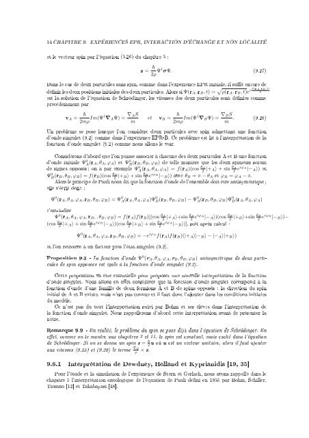
14 CHAPITRE 9. EXPÉRIENCES EPR, INTERACTION D'ÉCHANGE ET NON LOCALITÉ
et le vecteur spin par l'équation (5.26) du chapitre 5 :
s = 2ρ Ψ† σΨ. (9.27)
Dans le cas de deux particules sans spin, comme dans l'expérience EPR initiale, il sut encore de
dénir les deux positions initiales des deux particules. Alors si Ψ(r A ,r B , t) = √ ρ(r A ,r B , t)e i S(r ,r A B ,t)
est la solution de l'équation de Schrôdinger, les vitesses des deux particules sont dénies comme
précèdemment par
v A =
2mρ Im(Ψ† ∇ A Ψ) = ∇ AS
m
et v B =
2mρ Im(Ψ† ∇ B Ψ) = ∇ BS
m . (9.28)
Un problème se pose lorsque l'on considère deux particules avec spin admettant une fonction
d'onde singulet (9.2) comme dans l'expérience EPR-B. Ce problème est lié à l'interprétation de la
fonction d'onde singulet (9.2) comme nous allons le voir.
Considérons d'abord que l'on puisse associer à chacune des deux particules A et B une fonction
d'onde initiale Ψ 0 A (r A, θ A , ϕ A ) et Ψ 0 B (r B, θ B , ϕ B ) de telle manière que les deux spineurs soient
de signes opposés; on a par exemple Ψ 0 A (r A, θ A , ϕ A ) = f(r A )(cos θ A
2
|+ A 〉 + sin θ A
2
e iϕ A
|− A 〉) et
Ψ 0 B (r B, θ B , ϕ B ) = f(r B )(cos θ B
2
|+ B 〉 + sin θ B
2
e iϕ B
|− B 〉) avec θ B = π − θ A et ϕ B = ϕ A − π.
Alors le principe de Pauli nous dit que la fonction d'onde de l'ensemble doit être antisymétrique;
elle s'écrit donc :
Ψ 0 (r A , θ A , ϕ A ,r B , θ B , ϕ B ) = Ψ 0 A(r A , θ A , ϕ A )Ψ 0 B(r B , θ B , ϕ B ) − Ψ 0 A(r B , θ B , ϕ B )Ψ 0 B(r A , θ A , ϕ A )
c'est-à-dire
Ψ 0 (r A , θ A , ϕ A ,r B , , θ B , ϕ B ) = f(r A )f(r B )[(cos θ A
2
|+ A 〉+sin θ A
2
e iϕ A
|− A 〉)(cos θ B
2
|+ B 〉+sin θ B
2
e iϕ B
|− B 〉)−
(cos θ B
2
|+ A 〉 + sin θ B
2
e iϕ B
|− A 〉)(cos θ A
2
|+ B 〉 + sin θ A
2
e iϕ A
|− B 〉)], soit après calcul :
Ψ 0 (r A , θ A , ϕ A ,r B , θ B , ϕ B ) = −e iϕ A
f(r A )f(r B )(|+ A 〉|− B 〉 − |− A 〉|+ B 〉)
et l'on retrouve à un facteur près l'état singulet (9.2).
Proposition 9.3 - La fonction d'onde Ψ 0 (r A , θ A , ϕ A ,r B , θ B , ϕ B ) antisymétrique de deux particules
de spin opposées est égale à la fonction d'onde singulet (9.2).
Cette proposition va être essentielle pour proposer une nouvelle interprétation de la fonction
d'onde singulet. Nous allons en eet considérer que la fonction d'onde singulet correspond à la
fonction d'onde d'une famille de deux fermions A et B de spins opposés : la direction du spin
initial de A et B existe, mais n'est pas connue et il faut donc l'ajouter dans les conditions initiales
du modèle.
Ce n'est pas du tout l'interprétation suivi par Bohm et ses élèves dans l'interprétation de
la fonction d'onde singulet. Nous rappellerons d'abord cette interprétation avant de présenter la
nôtre.
Remarque 9.9 - En réalité, le problème du spin se pose déjà dans l'équation de Schrödinger. En
eet, comme on le montre aux chapitres 3 et 11, le spin est constant, mais caché dans l'équation
de Schrödinger. Si on se donne un spin s = 2u où u est un vecteur unitaire, alors il faut ajouter
aux vitesses (9.25) et (9.28) le terme ∇ρ
ρ × s.
9.6.1 Interprétation de Dewdney, Holland et Kyprianidis [19, 35]
Pour l'étude et la simulation de l'expérience de Stern et Gerlach, nous avons rappellé dans le
chapitre 5 l'interprétation ontologique de l'équation de Pauli déni en 1955 par Bohm, Schiller,
Tiomno [12] et Takabayasi [48].