
You also want an ePaper? Increase the reach of your titles
YUMPU automatically turns print PDFs into web optimized ePapers that Google loves.
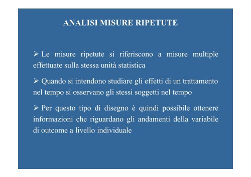
<strong>ANALISI</strong> <strong>MISURE</strong> <strong>RIPETUTE</strong><br />
‣ Le misure ripetute si riferiscono a misure multiple<br />
effettuate sulla stessa unità statistica<br />
‣ Quando si intendono studiare gli effetti di un trattamento<br />
nel tempo si osservano gli stessi soggetti nel tempo<br />
‣ Per questo tipo di disegno è quindi possibile ottenere<br />
informazioni che riguardano gli andamenti della variabile<br />
di outcome a livello individuale
Soggetto<br />
Tempo<br />
Risposta<br />
1<br />
i<br />
n<br />
1<br />
j<br />
t 1<br />
1<br />
j<br />
t i<br />
1<br />
j<br />
t n<br />
Y 11<br />
Y 1j<br />
Y 1t1<br />
Y i1<br />
Y ij<br />
Y iti<br />
Y n 1<br />
Y n j<br />
Y n tn
• In generale si osserva una certa correlazione tra<br />
misure differenti sullo stesso soggetto e quindi la<br />
risposta ad un certo tempo non potrà essere<br />
indipendente dalla risposta ad un tempo precedente<br />
• Esempio: intendo confrontare l’effetto di un certo<br />
farmaco rispetto a placebo e misuro ad esempio la<br />
risposta al trattamento all’inizio del trattamento, alla<br />
fine del trattamento e dopo un certo periodo di tempo<br />
dall’inizio del trattamento
• Posso limitarmi a confrontare le medie dei valori<br />
al termine del follow-up<br />
• Ci potrebbe essere un diverso comportamento nel<br />
tempo dell’efficacia del farmaco rispetto al<br />
placebo e quindi posso essere interessato a come<br />
variano le medie dei due trattamenti nei diversi<br />
tempi
Tratto da Dott.ssa Zambon: Modelli Statistici per le sperimentazioni<br />
cliniche – Milano Bicocca
Tempo<br />
terapia<br />
paziente<br />
0<br />
1<br />
…<br />
t<br />
1<br />
1<br />
i<br />
n 1<br />
y 110<br />
…<br />
y 1n10<br />
y 111<br />
…<br />
y 1n11<br />
…<br />
…<br />
…<br />
y 11t<br />
…<br />
y 1n1t<br />
h<br />
1<br />
i<br />
n h<br />
y h10<br />
…<br />
y hnh0<br />
y h11<br />
…<br />
y hnh1<br />
…<br />
…<br />
…<br />
y h1t<br />
…<br />
y hnht<br />
s<br />
1<br />
i<br />
n s<br />
y s10<br />
…<br />
Y sns0<br />
y s11<br />
…<br />
Y sns1<br />
…<br />
…<br />
…<br />
y s1t<br />
…<br />
Y snst
Metodo univariato<br />
• L’approccio più semplice per l’analisi delle misure ripetute<br />
è quello di ridurre il vettore delle misure di ogni unità<br />
sperimentale in modo tale che la variabile risposta sia una<br />
sola:<br />
Soggetto tempo<br />
risposta<br />
1 1 …<br />
1 2 …<br />
1 3 …<br />
2 1 …<br />
2 2 …<br />
2 3 …
Esempio<br />
6,0<br />
5,0<br />
4,0<br />
3,0<br />
gruppo1<br />
gruppo2<br />
2,0<br />
1,0<br />
0,0<br />
1 2 3<br />
tempi
isposta = terapia paziente(terapia) tempo terapia*tempo<br />
(effetto paziente: assumiamo che c’è una variabilità del<br />
paziente all’interno del livello terapia)<br />
Origine<br />
DF<br />
Somma dei<br />
quadrati<br />
Media<br />
quadratica<br />
Valore<br />
F<br />
Pr > F<br />
Model 33 343.1892706 10.3996749 36.05
Metodo univariato<br />
Origine DF Type III SS<br />
Media<br />
quadratica<br />
Valore<br />
F<br />
Pr > F<br />
effetto terapia 1 6.83071639 6.83071639 4.44 0.0441<br />
Pazienti(terapia) 28 43.0441331 1.5372905 5.33
• Abbiamo trattato la risposta in modo “univariato”<br />
assumendo che le correlazioni tra i diversi tempi siano<br />
uguali<br />
• Questo assunto potrebbe essere poco realistico<br />
soprattutto se l’esperimento ha tempi di rilevazione<br />
alla risposta non equispaziati o se il tempo<br />
dell’esperimento è molto lungo.<br />
• Approccio multivariato
Approccio multivariato<br />
• La variabile di risposta è un vettore di risposte<br />
model tempo1 tempo2 tempo3 tempo4=terapia<br />
The GLM Procedure<br />
Repeated Measures Analysis of Variance<br />
MANOVA Test Criteria and Exact F Statistics for the Hypothesis of no time Effect<br />
Statistic Value F Value Num DF Den DF Pr > F<br />
Wilks' Lambda 0.23333404 2.19 3 2 0.3287<br />
Pillai's Trace 0.76666596 2.19 3 2 0.3287<br />
Hotelling-Lawley Trace 3.28570126 2.19 3 2 0.3287<br />
Roy's Greatest Root 3.28570126 2.19 3 2 0.3287<br />
MANOVA Test Criteria and Exact F Statistics for the Hypothesis of no time*group Effect<br />
Statistic Value F Value Num DF Den DF Pr > F<br />
Wilks' Lambda 0.77496006 0.19 3 2 0.8932<br />
Pillai's Trace 0.22503994 0.19 3 2 0.8932<br />
Hotelling-Lawley Trace 0.29038909 0.19 3 2 0.8932<br />
Roy's Greatest Root 0.29038909 0.19 3 2 0.8932
Repeated Measures Analysis of Variance<br />
Analysis of Variance of Contrast Variables<br />
time_N represents the nth successive difference in time<br />
Contrast Variable: time_1<br />
Time1 vs. time2<br />
Source DF Type III SS Mean Square F Value Pr > F<br />
Mean 1 6.00000000 6.00000000 0.35 0.5879<br />
group 1 16.66666667 16.66666667 0.96 0.3823<br />
Error 4 69.33333333 17.33333333<br />
Contrast Variable: time_2<br />
Time2 vs. time3<br />
Source DF Type III SS Mean Square F Value Pr > F<br />
Mean 1 192.6666667 192.6666667 2.56 0.1850<br />
group 1 6.0000000 6.0000000 0.08 0.7918<br />
Error 4 301.3333333 75.3333333<br />
Contrast Variable: time_3<br />
Time3 vs. time4<br />
Source DF Type III SS Mean Square F Value Pr > F<br />
Mean 1 433.5000000 433.5000000 9.06 0.0395<br />
group 1 0.1666667 0.1666667 0.00 0.9558<br />
Error 4 191.3333333 47.8333333