Cenni Teorici “Scienza delle Costruzioni” - Polihelp.com

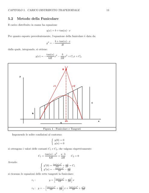
CAPITOLO 5. CARICO DISTRIBUITO TRAPEZOIDALE 13
5.2 Metodo della Funicolare
Il carico distribuito in esame ha equazione
q(x) = b + tan(α) · x
Per quanto esposto precedentemente, l’equazione della funicolare è data da:
dalla quale, integrando, si ottiene:
y ′′ b + tan(α) · x
= −
H
y(x) = − tan(α)
6H x3 − b
2H x2 + C1x + C2
Figura 4 - Funicolare e Tangenti
Imponendo le solite condizioni al contorno:
� y(0) = 0
y(a) = 0
si ottengono i valori delle costanti C1 e C2, che valgono rispettivamente:
C1 =
Avendo: �
tan(α) · a2
6H
+ a · b
y ′ (0) = tan(α)·a2
6H
2H
y ′ (a) = − tan(α)·a2
3H
a·b + 2H
C2 = 0
= C1
a·b −
si ricavano le equazioni delle rette tangenti la funicolare:
� �
tan(α)·a2 a·b
r1 : y = + x
�
tan(α)·a2 r2 : y = − 3H
6H
a·b +
2H
2H
2H
�
x + tan(α)·a3
3H + a2 ·b
2H