Capítulo 22 - Instituto de Matemática - UFRJ

More documents

Recommendations

Info

304 Cap. 22. O Teorema Fundamental do Cálculo e Integrais Indefinidas 4. Este teorema torna o difícil problema de calcular integrais definidas por meio do cálculo do limite de somas num problema muito mais fácil de encontrar primitivas. Portanto, para achar o valor de ∫ b f(x) dx não precisamos a mais calcular limites de somas de Riemann; simplesmente achamos, da maneira que for possível (por inspeção, por algum cálculo inteligente, por inspiração divina, procurando numa tabela, usando o Maple), uma primitiva F da função que queremos integrar e calculamos o número F (b) − F (a). 5. A tarefa de encontrar primitivas de funções não é trivial e, em alguns casos, é impossível determinar primitivas em termos de funções elementares – polinômios, senos e cossenos, logaritmos e exponenciais, ou combinações e composições destas funções. No entanto, a função A(x) definida no teorema fundamental do cálculo, existe sempre que o integrando for uma função contínua no intervalo [a, x], mesmo que não saibamos calculá-la explicitamente, e é contínua, pois é derivável. Neste sentido, por exemplo, o problema de se achar uma fórmula explícita para a integral ∫ x a sen(x 2 ) dx está fora do nosso alcance. Entretanto, se em vez de procurarmos uma fórmula explícita para esta integral quisermos apenas uma função bem definida, a expressão F (x) = ∫ x a sen(x2 ) dx servirá como uma boa definição para a função procurada. (Veja o Exemplo 5.) Exemplo 1 Se n é um inteiro positivo, calcule uma primitiva de x n e use este resultado para calcular ∫ 2 −1 x5 dx. Solução Como d ( ) (n+1) x dx n + 1 cálculo obtemos: Exemplo 2 Calcule ∫ 2 −1 = x n , temos que x6 6 ∫ 2 −1 x 2 − x dx . x 5 dx = x6 6 2 é a primitiva procurada. Assim, pelo teorema fundamental do −1 = 26 6 − (−1)6 6 = 63 6 . Solução: Como x 2 − x ≤ 0 em (0, 1) e x 2 − x ≥ 0 em (−1, 0) e (1, 2), usando as propriedades da integral definida, temos ∫ 2 −1 x 2 − x dx = = ∫ 0 −1 [ x 3 3 = −( (−1)3 3 x 2 − x dx + ]0 x2 − + 2 −1 ∫ 1 0 [ x 2 2 (−1)2 − ) + ( 2 1 2 x − x 2 dx + ]1 x3 − + 3 0 Exemplo 3 Considere a função f(x) = 2 x3 + 2 x2 − 4 x . (a) Calcule ∫ 1 f(x) dx. −2 (b) Ache a área da região limitada pelo gráfico de f e o eixo x. Solução (a) Como a função F (x) = x4 f(x) = 2 x 3 + 2 x 2 − 4 x, tem-se que ∫ 1 −2 2 x 3 + 2 x 2 − 4 x dx = x4 2 2 ∫ 2 1 [ x 3 3 x 2 − x dx ]2 x2 − 2 1 1 22 − ) + [23 − − (1 3 3 2 3 + 2 x3 3 − 2 x2 é uma primitiva de + 2 x3 3 (b) Observe o o seguinte gráfico da função f: − 2 x2 1 −2 1 11 − )] = 2 6 . = 1 2 2 (−2)3 + − 2 − ((−2)4 + − 2 (−2) 2 3 2 3 2 ) = 9 2
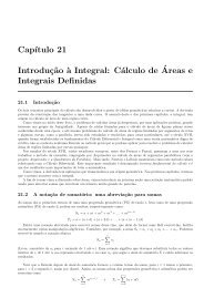
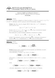
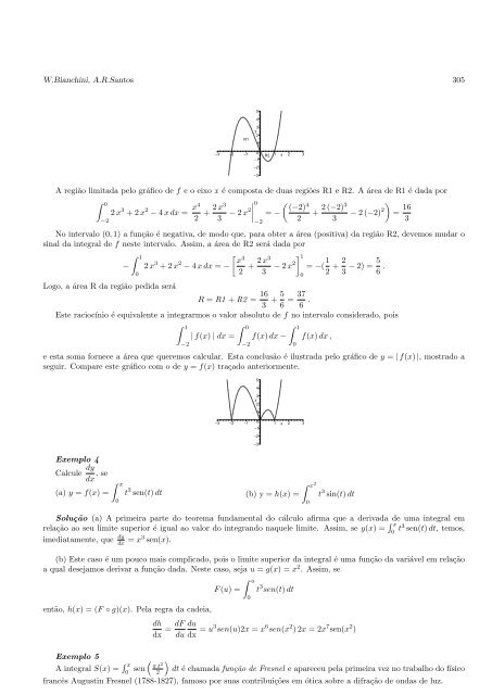
W.Bianchini, A.R.Santos 305 R1 5 4 3 y 2 1 –3 –2 –1 0 –1 R2 1 x 2 3 A região limitada pelo gráfico de f e o eixo x é composta de duas regiões R1 e R2. A área de R1 é dada por ∫ 0 2 x 3 + 2 x 2 − 4 x dx = x4 0 ( 2 x3 4 + − 2 x2 (−2) 2 (−2)3 2 3 = − + − 2 (−2) 2 3 2 ) = 16 3 −2 –2 –3 No intervalo (0, 1) a função é negativa, de modo que, para obter a área (positiva) da região R2, devemos mudar o sinal da integral de f neste intervalo. Assim, a área de R2 será dada por ∫ 1 − 2 x 3 + 2 x 2 [ ]1 4 x 2 x3 − 4 x dx = − + − 2 x2 = −( 2 3 1 2 5 + − 2) = 2 3 6 . 0 Logo, a área R da região pedida será R = R1 + R2 = 16 5 37 + = 3 6 6 . Este raciocínio é equivalente a integrarmos o valor absoluto de f no intervalo considerado, pois ∫ 1 −2 | f(x) | dx = ∫ 0 −2 −2 f(x) dx − ∫ 1 0 0 f(x) dx , e esta soma fornece a área que queremos calcular. Esta conclusão é ilustrada pelo gráfico de y = | f(x) |, mostrado a seguir. Compare este gráfico com o de y = f(x) traçado anteriormente. Exemplo 4 Calcule dy , se dx (a) y = f(x) = ∫ x 0 5 4 3 y 2 1 –3 –2 –1 0 –1 1 x 2 3 t 3 sen(t) dt (b) y = h(x) = –2 –3 ∫ x 2 0 t 3 sin(t) dt Solução (a) A primeira parte do teorema fundamental do cálculo afirma que a derivada de uma integral em relação ao seu limite superior é igual ao valor do integrando naquele limite. Assim, se y(x) = ∫ x 0 t3 sen(t) dt, temos, imediatamente, que dy dx = x3 sen(x). (b) Este caso é um pouco mais complicado, pois o limite superior da integral é uma função da variável em relação a qual desejamos derivar a função dada. Neste caso, seja u = g(x) = x2 . Assim, se então, h(x) = (F ◦ g)(x). Pela regra da cadeia, F (u) = ∫ u 0 t 3 sen(t) dt dh dF du = dx du dx = u3sen(u)2x = x 6 sen(x 2 ) 2x = 2x 7 sen(x 2 ) Exemplo 5 A integral S(x) = ∫ x 0 sen ( ) 2 π t 2 dt é chamada função de Fresnel e apareceu pela primeira vez no trabalho do físico francês Augustin Fresnel (1788-1827), famoso por suas contribuições em ótica sobre a difração de ondas de luz.
Page 1 and 2: Capítulo 22 O Teorema Fundamental
Page 3: W.Bianchini, A.R.Santos 303 Como x
Page 7 and 8: W.Bianchini, A.R.Santos 307 Em gera
Page 9 and 10: W.Bianchini, A.R.Santos 309 6. Para
Page 11 and 12: W.Bianchini, A.R.Santos 311 4 3 2 1
Page 13 and 14: W.Bianchini, A.R.Santos 313 movimen

Capítulo 22 - Instituto de Matemática - UFRJ

You also want an ePaper? Increase the reach of your titles

Delete template?

Save as template?