SBP Working Paper Series STATE BANK OF PAKISTAN
n?u=RePEc:sbp:wpaper:74&r=mon
n?u=RePEc:sbp:wpaper:74&r=mon
You also want an ePaper? Increase the reach of your titles
YUMPU automatically turns print PDFs into web optimized ePapers that Google loves.
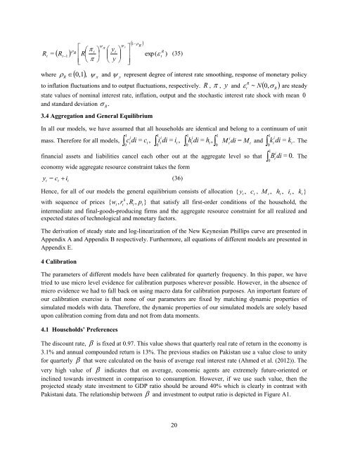
R<br />
t<br />
=<br />
<br />
R<br />
t1<br />
<br />
<br />
R<br />
<br />
t <br />
R<br />
<br />
<br />
<br />
<br />
R<br />
<br />
<br />
<br />
where 0,1,<br />
and<br />
<br />
yt<br />
<br />
<br />
y <br />
y<br />
<br />
<br />
<br />
<br />
1<br />
R<br />
<br />
R<br />
exp( )<br />
t<br />
(35)<br />
<br />
y<br />
represent degree of interest rate smoothing, response of monetary policy<br />
R<br />
to inflation fluctuations and to output fluctuations, respectively. R , , y and 0,<br />
<br />
t<br />
~ N <br />
R<br />
are steady<br />
state values of nominal interest rate, inflation, output and the stochastic interest rate shock with mean 0<br />
and standard deviation <br />
R.<br />
3.4 Aggregation and General Equilibrium<br />
In all our models, we have assumed that all households are identical and belong to a continuum of unit<br />
1<br />
1<br />
1<br />
1<br />
1<br />
i<br />
i<br />
i<br />
i<br />
i<br />
mass. Therefore for all models, ct<br />
di = ct<br />
, it<br />
di = it<br />
, h<br />
t<br />
di = h t<br />
, M<br />
t<br />
di = Mt<br />
and kt<br />
di = kt.<br />
The<br />
0<br />
0<br />
financial assets and liabilities cancel each other out at the aggregate level so that B i t<br />
di = 0. The<br />
0<br />
economy wide aggregate resource constraint takes the form<br />
y = c i<br />
(36)<br />
t<br />
t<br />
t<br />
Hence, for all of our models the general equilibrium consists of allocation { y t<br />
,<br />
0<br />
0<br />
t<br />
0<br />
1<br />
c , M , h , i , k }<br />
k<br />
with sequence of prices { w<br />
t,<br />
rt<br />
, Rt<br />
, pt}<br />
that satisfy all first-order conditions of the household, the<br />
intermediate and final-goods-producing firms and the aggregate resource constraint for all realized and<br />
expected states of technological and monetary factors.<br />
The derivation of steady state and log-linearization of the New Keynesian Phillips curve are presented in<br />
Appendix A and Appendix B respectively. Furthermore, all equations of different models are presented in<br />
Appendix E.<br />
4 Calibration<br />
The parameters of different models have been calibrated for quarterly frequency. In this paper, we have<br />
tried to use micro level evidence for calibration purposes wherever possible. However, in the absence of<br />
micro evidence we had to fall back on using macro data for calibration purposes. An important feature of<br />
our calibration exercise is that none of our parameters are fixed by matching dynamic properties of<br />
simulated models with data. Therefore, the dynamic properties of our simulated models are solely based<br />
upon calibration coming from data and not from data moments.<br />
4.1 Households’ Preferences<br />
The discount rate, is fixed at 0.97. This value shows that quarterly real rate of return in the economy is<br />
3.1% and annual compounded return is 13%. The previous studies on Pakistan use a value close to unity<br />
for quarterly that were calculated on the basis of average real interest rate (Ahmed et al. (2012)). The<br />
very high value of indicates that on average, economic agents are extremely future-oriented or<br />
inclined towards investment in comparison to consumption. However, if we use such value, then the<br />
projected steady state investment to GDP ratio should be around 40% which is clearly in contrast with<br />
Pakistani data. The relationship between and investment to output ratio is depicted in Figure A1.<br />
t<br />
t<br />
t<br />
t<br />
20


