

Economic, Revenue and Spending Methodologies - New York State ...
Economic, Revenue and Spending Methodologies - New York State ...
Economic, Revenue and Spending Methodologies - New York State ...

You also want an ePaper? Increase the reach of your titles
YUMPU automatically turns print PDFs into web optimized ePapers that Google loves.
Level<br />
<strong>New</strong> <strong>York</strong> <strong>State</strong><br />
110<br />
105<br />
100<br />
95<br />
90<br />
85<br />
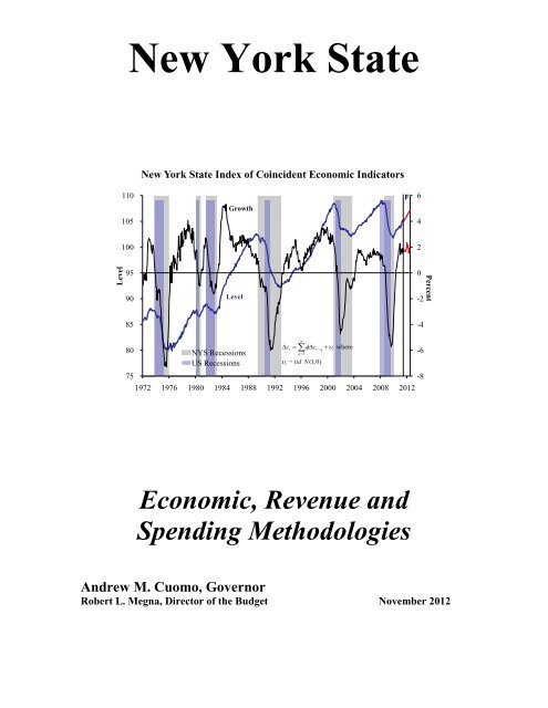
<strong>New</strong> <strong>York</strong> <strong>State</strong> Index of Coincident <strong>Economic</strong> Indicators<br />
Growth<br />
Level<br />
80<br />
NYS Recessions<br />
∆ ct= ∑φ∆<br />
ct−q<br />
+ υtwhere<br />
q=<br />
1<br />
-6<br />
US Recessions<br />
υt<br />
~ iid N(1,<br />
0)<br />
75<br />
-8<br />
1972 1976 1980 1984 1988 1992 1996 2000 2004 2008 2012<br />
<strong>Economic</strong>, <strong>Revenue</strong> <strong>and</strong><br />
<strong>Spending</strong> <strong>Methodologies</strong><br />
Andrew M. Cuomo, Governor<br />
Robert L. Megna, Director of the Budget November 2012<br />
n<br />
F<br />
6<br />
4<br />
2<br />
0<br />
-2<br />
-4<br />
Percent
TABLE OF CONTENTS<br />
OVERVIEW OF THE METHODOLOGY PROCESS 1<br />
PART I - ECONOMIC METHODOLOGIES<br />
United <strong>State</strong>s Macroeconomic Model ........................................................................ 17<br />
<strong>New</strong> <strong>York</strong> <strong>State</strong> Macroeconomic Model ................................................................... 49<br />
<strong>New</strong> <strong>York</strong> <strong>State</strong> Adjusted Gross Income ................................................................... 57<br />
References .................................................................................................................. 68<br />
PART II - REVENUE METHODOLOGIES<br />
Personal Income Tax.................................................................................................. 71<br />
User Taxes <strong>and</strong> Fees<br />
Sales <strong>and</strong> Use Tax ................................................................................................ 93<br />
Cigarette <strong>and</strong> Tobacco Taxes ...............................................................................101<br />
Motor Fuel Tax ....................................................................................................106<br />
Alcoholic Beverage Taxes .................................................................................108<br />
Highway Use Tax ................................................................................................111<br />
Business Taxes<br />
Bank Tax ..............................................................................................................114<br />
Corporation Franchise Tax ..................................................................................121<br />
Corporation <strong>and</strong> Utilities Taxes ...........................................................................130<br />
Insurance Taxes ...................................................................................................136<br />
Petroleum Business Taxes ...................................................................................142<br />
Other Taxes<br />
Estate Tax.............................................................................................................145<br />
Real Estate Transfer Tax ......................................................................................151<br />
Pari-Mutuel Taxes ................................................................................................155<br />
Lottery ........................................................................................................................158<br />
Video Lottery .............................................................................................................168<br />
Mobility Tax ..............................................................................................................179<br />
PART III - SPENDING METHODOLOGIES<br />
School Aid .................................................................................................................182<br />
Medicaid ....................................................................................................................185<br />
Welfare .......................................................................................................................193<br />
Child Welfare .............................................................................................................198<br />
Debt Service ...............................................................................................................201<br />
Personal Service .........................................................................................................208<br />
Non Personal Service .................................................................................................215<br />
Employee <strong>and</strong> Retiree Health Insurance ....................................................................222<br />
Pensions .....................................................................................................................225
AN OVERVIEW OF THE<br />
METHODOLOGY PROCESS<br />
The Division of the Budget (DOB) <strong>Economic</strong>, <strong>Revenue</strong> <strong>and</strong> <strong>Spending</strong> <strong>Methodologies</strong><br />
supplements the detailed forecast of the economy, tax, <strong>and</strong> spending forecasts presented<br />
in the Executive Budget <strong>and</strong> Quarterly Updates. The purpose of this volume is to provide<br />
background information on the methods <strong>and</strong> models used to generate the estimates for the<br />
major receipt <strong>and</strong> spending sources contained in the 2012-13 Mid-Year Update <strong>and</strong> the<br />
upcoming 2013-14 Executive Budget. DOB’s forecast methodology utilizes<br />
sophisticated econometric models, augmented by the input of a panel of economic<br />
experts, <strong>and</strong> a thorough review of economic, revenue <strong>and</strong> spending data to form multiyear<br />
quarterly projections of economic, revenue, <strong>and</strong> spending changes.<br />
The spending side analysis is designed to provide, in summary form, background<br />
information on the methods <strong>and</strong> analyses used to generate the spending estimates for a<br />
number of major program areas contained in the budget, <strong>and</strong> is meant to enhance the<br />
presentation <strong>and</strong> transparency of the <strong>State</strong>’s spending forecast. The methodologies<br />
illustrate how spending forecasts are the product of many factors <strong>and</strong> sources of<br />
information, including past performance <strong>and</strong> trends, administrative constraints, expert<br />
judgment of agency staff, <strong>and</strong> information in the <strong>State</strong>’s economic analysis <strong>and</strong> forecast,<br />
especially in cases where spending trends are sensitive to changes in economic<br />
conditions.<br />
AN ASSESSMENT OF FORECAST RISK<br />
No matter how sophisticated the methods used, all forecasts are subject to error. For<br />
this reason, a proper assessment of the most significant forecast risks can be as critical to<br />
the budget process as the forecast itself. Therefore, we begin by reviewing the most<br />
important sources of forecast error <strong>and</strong> discuss how they affect the spending <strong>and</strong> receipt<br />
forecasts used to construct the Mid-Year Update.<br />
Data Quality<br />
Even the most accurate forecasting model is constrained by the accuracy of the<br />
available data. The data used by the Budget Division to produce a forecast typically<br />
undergo several stages of revision. For example, the quarterly components of real U.S.<br />
gross domestic product (GDP), the most widely cited measure of national economic<br />
activity, are revised no less than five times over a four-year period, not including the<br />
rebasing process. Each revision incorporates data that were not available when the prior<br />
estimate was made. Initial estimates are often based on sample information, though early<br />
vintages are sometimes based on the informed judgment of the analyst charged with<br />
tabulating the data. The monthly employment estimates produced under the Current<br />
Employment Statistics (CES) program undergo a similar revision process as better, more<br />
broad-based data become available <strong>and</strong> with the evolution of seasonal factors. For<br />
example, the total U.S. nonagricultural employment estimate for December 1989 has<br />
been revised no less than ten times since it was first published in January 1990. 1 Less<br />
1<br />
The current estimate for total employment for December 1989 of 108.8 million is 0.7 percent below the<br />
initial estimate of 109.5 million.<br />
1
AN OVERVIEW OF THE METHODOLOGY PROCESS<br />
frequently, data are revised based on new definitions of the underlying concepts. 2<br />
Unfortunately, revisions tend to be largest at or near business cycle turning points, when<br />
accuracy is most critical to fiscal planners. Finally, as demonstrated below, the available<br />
data are sometimes not suitable for economic or revenue forecasting purposes, such as the<br />
U.S. Bureau of <strong>Economic</strong> Analysis estimate of wages at the state level.<br />
Model Specification Error<br />
<strong>Economic</strong> forecasting models are by necessity simplifications of complex social<br />
processes involving millions of decisions made by independent agents. Although<br />
economic <strong>and</strong> fiscal policy theory provides some guidance as to how these models should<br />
be specified, theory is often imprecise with respect to capturing behavioral dynamics <strong>and</strong><br />
structural shifts. Moreover, modeled relationships may vary over time. Often one must<br />
choose between models that use the average behavior of the series over its entire history<br />
to forecast the future <strong>and</strong> models which give more weight to the more recent behavior of<br />
the series. Although more complicated models may do a better job of capturing history,<br />
they may be no better at forecasting the future, leading to the parsimony principle as a<br />
guiding precept in the model building process.<br />
Reporting Model Coefficients: Fixed Points or Ranges?<br />
Although model coefficients are generally treated as fixed in the forecasting process,<br />
coefficient estimates are themselves r<strong>and</strong>om variables, governed by probability<br />
distributions. Typically, the error distribution is assumed to be normal, a key to making<br />
statistical inference. Reporting the st<strong>and</strong>ard errors of the coefficient distributions gives<br />
some indication of how precisely one can measure the relationship between two<br />
variables. For many of the results reported below, point estimates of the coefficients are<br />
reported along with their st<strong>and</strong>ard errors. However, it would be more accurate to say that<br />
there is a 66 percent probability that the true coefficient lies within a range of the<br />
estimated coefficient plus <strong>and</strong> minus the st<strong>and</strong>ard error.<br />
<strong>Economic</strong> Shocks<br />
No model can adequately capture the multitude of r<strong>and</strong>om events occur that can<br />
affect the economy, <strong>and</strong> hence revenue <strong>and</strong> spending results. September 11 is an<br />
example of such an event. Also, some economic variables are more sensitive to shocks<br />
than others. For example, equity markets rise <strong>and</strong> fall on the day’s news, sometimes by<br />
large magnitudes. In contrast, GDP growth tends to fluctuate within a relatively narrow<br />
range. For all of these reasons, the probability of any forecast being precisely accurate is<br />
virtually zero. But although one cannot be confident about hitting any particular number<br />
correctly, one can feel more confident about specifying a range within which the actual<br />
number is likely to fall. Often economic forecasters use sophisticated techniques, such as<br />
Monte Carlo analysis, to estimate confidence b<strong>and</strong>s based on model performance, the<br />
precision of the coefficient estimates, <strong>and</strong> the inherent volatility of the series. A 95<br />
percent confidence b<strong>and</strong> (or even a much less exacting b<strong>and</strong>) often can be quite wide,<br />
2 The switch from SIC to NAICS is a classic example of how changes in the definition of a data series can<br />
challenge the modeler. The switch not only changed the industrial classification scheme, but also robbed<br />
state modelers of decades of employment history.<br />
2
AN OVERVIEW OF THE METHODOLOGY PROCESS<br />
suggesting the possibility that the actual result could deviate substantially from the point<br />
estimate. Even with a 95 percent b<strong>and</strong>, there is a 5 percent chance of a shock that results<br />
in an extremely unexpected outcome. Indeed, based on some of the events of the last 10<br />
years — the high-tech/Internet bubble, September 11, <strong>and</strong> the recent financial crisis — it<br />
could be argued that this probability is much higher than 5 percent. Finally, from a<br />
practitioner’s perspective, these techniques are only valid if the model is properly<br />
specified.<br />
What sometimes appears to be a r<strong>and</strong>om economic shock may actually be a more<br />
permanent structural change. Shifts in the underlying economic, revenue, or spending<br />
structure are difficult to model in practice, particularly since the true causes of such shifts<br />
only become clear with hindsight. This can lead to large forecast errors when these shifts<br />
occur rapidly or when the cumulative impact is felt over the forecast horizon. Policy<br />
makers must be kept aware that even a well specified model can perform badly when<br />
structural changes occur.<br />
Evaluating a Loss Function<br />
The prevalence of sources of forecast error underscores the importance of assessing<br />
the risks to the forecast, <strong>and</strong> explains why the discussion of such risks consumes such a<br />
large portion of the economic backdrop presented with the Executive Budget. In light of<br />
all of the potential sources of forecast risk, how does a budgeting entity utilize the<br />
knowledge of risks to inform the forecast? St<strong>and</strong>ard econometric theory tells us that the<br />
probability of any point forecast being correct is virtually zero, but a budget must be<br />
based on a single projection.<br />
One way to reconcile these two facts is to evaluate the cost of one’s forecasting<br />
errors, giving rise to the notion of a loss function. A conventional example of a loss<br />
function is the root-mean-squared forecast error (RMSFE). In constructing that measure,<br />
the “cost” of an inaccurate forecast is the square of the forecast error itself, implying that<br />
large forecast errors are weighted more heavily than small errors. Because positive <strong>and</strong><br />
negative errors of equal magnitude are weighted the same, the RMSFE is symmetric.<br />
However, in the world of professional forecasting, as in our daily lives, the costs<br />
associated with an inaccurate forecast may not truly be symmetric. For example, how<br />
much time we give ourselves to get to the airport may not be based on the average travel<br />
time between home <strong>and</strong> the gate, since the cost of being late <strong>and</strong> missing the plane may<br />
outweigh the cost of arriving early <strong>and</strong> waiting awhile longer. Granger <strong>and</strong> Pesaran<br />
(2000) show that the forecast evaluation criterion derived from a decision-based approach<br />
can differ markedly from the usual RMSFE. They suggest a more general approach,<br />
known as generalized cost-of-error functions, to deal with asymmetries in the cost of<br />
over- <strong>and</strong> under-predicting. 3 In the revenue-estimating context, the cost of<br />
overestimating receipts for a fiscal year may outweigh the cost of underestimating<br />
receipts, given that ongoing spending decisions may be based on revenue resources<br />
projected to be available. In summary, errors are an inevitable part of the forecasting<br />
process <strong>and</strong>, as a result, policymakers must be fully informed of the forecast risks, both as<br />
to direction <strong>and</strong> magnitude.<br />
3 For a detailed discussion, see C.W.J. Granger, Empirical Modeling in <strong>Economic</strong>s: Specification <strong>and</strong><br />
Evaluation, Cambridge University Press, 1999.<br />
3
AN OVERVIEW OF THE METHODOLOGY PROCESS<br />
The flow chart below provides an overview of the receipts forecasting process (an<br />
equivalent spending chart is included below). The entire forecast process, from the<br />
gathering of information to the running of various economic <strong>and</strong> receipt models, is<br />
designed to inform <strong>and</strong> improve the DOB receipt estimates. As with any large scale<br />
forecasting process, the qualitative judgment of experts plays an important role in the<br />
estimation process. It is the job of the DOB economic <strong>and</strong> revenue analysts to consider<br />
all of the sources of model errors <strong>and</strong> to assess the impact of changes in the revenue<br />
environment that models cannot be expected to capture. Adjustments that balance all of<br />
these risks while minimizing the appropriate loss function are key elements of the<br />
process. Nevertheless, in the final analysis, such adjustments tend to be relatively small.<br />
The Budget Division’s forecasting process remains guided primarily by the results from<br />
the models described in detail below.<br />
Blue Chip<br />
Global Insight<br />
Analysis<br />
Macroeconomic<br />
Advisers<br />
Moody’s<br />
Economy.com<br />
Treasury OMB<br />
CBO<br />
Outside<br />
<strong>Economic</strong><br />
Forecasts<br />
Tax & Finance<br />
OSC<br />
Receipt<br />
Lottery Data<br />
DMV<br />
Banking Department<br />
Insurance Department<br />
The <strong>Economic</strong> <strong>and</strong> <strong>Revenue</strong> Forecasting Process<br />
Income Tax<br />
Simulation<br />
*Study Files Include:<br />
- Income Tax<br />
- Corporate Franchise Tax<br />
- Bank Tax<br />
- Insurance Tax<br />
THE ECONOMY<br />
US Bureau of<br />
<strong>Economic</strong><br />
US Census<br />
Bureau<br />
Federal<br />
Reserve Board<br />
US Labor<br />
Department<br />
US<br />
<strong>Economic</strong><br />
Data<br />
DOB ADJUSTED<br />
GROSS INCOME<br />
MODEL<br />
Study<br />
Files*<br />
DOB U.S.<br />
MACRO-MODEL<br />
US<br />
FORECAST<br />
DOB N.Y.<br />
MODEL<br />
NY<br />
FORECAST<br />
RECEIPTS<br />
MODEL<br />
RECEIPT FORECAST<br />
Taxes, Miscellaneous Receipts, Lottery,<br />
Motor Vehicle Fees<br />
4<br />
NY<br />
<strong>Economic</strong><br />
Data<br />
Corporate Tax<br />
Simulation<br />
DOB<br />
<strong>Economic</strong><br />
Advisors<br />
US Bureau of<br />
<strong>Economic</strong><br />
Analysis<br />
NYS Labor<br />
Department<br />
Tax & Finance<br />
US Census<br />
Bureau<br />
Value Line<br />
St<strong>and</strong>ard & Poor’s<br />
Financial Reports<br />
Income <strong>State</strong>ments<br />
Macro<br />
Economy<br />
Finance<br />
Banking<br />
<strong>State</strong> Fiscal<br />
Condition<br />
Industry<br />
Studies<br />
The economic environment is the most important factor influencing the receipts<br />
estimates <strong>and</strong> has an important impact on spending decisions. <strong>New</strong> <strong>York</strong> <strong>State</strong>’s revenue<br />
base is dominated by tax sources, such as the personal income <strong>and</strong> sales taxes, that are<br />
sensitive to economic conditions. In addition, expenditures such as Medicaid, welfare,<br />
debt service, <strong>and</strong> nonpersonal service costs are directly related to the state of the<br />
economy. As a result, the first <strong>and</strong> most important step in the construction of receipts <strong>and</strong><br />
spending projections requires an analysis of economic trends at both the <strong>State</strong> <strong>and</strong><br />
national levels. The schedule below sketches the frequency <strong>and</strong> timing of forecasts<br />
performed over the course of the year.
AN OVERVIEW OF THE METHODOLOGY PROCESS<br />
ECONOMIC AND REVENUE FORECAST SCHEDULE<br />
A brief overview of how the Budget Division forecasting process unfolds over the course of the calendar year is<br />
presented below. From one perspective, the following schedule begins at the end, since the submission of the<br />
Executive Budget in January represents the culmination of research <strong>and</strong> analysis done throughout the preceding year.<br />
For the remainder of the year, the <strong>Economic</strong> <strong>and</strong> <strong>Revenue</strong> Unit closely monitors all of the relevant economic <strong>and</strong><br />
revenue data <strong>and</strong> regularly updates an extensive array of annual, quarterly, monthly, weekly, <strong>and</strong> daily databases. For<br />
example, estimates of U.S. Gross Domestic Product data are released at the end of each month for the preceding<br />
quarter. U.S. employment <strong>and</strong> unemployment rate data are released on the first Friday of each month for the<br />
preceding month, while unemployment benefits claims data are released on a weekly basis. Receipts data published<br />
by the Office of the <strong>State</strong> Comptroller are released by the 15th of each month for the preceding month, while similar<br />
data from the <strong>New</strong> <strong>York</strong> <strong>State</strong> Department of Taxation <strong>and</strong> Finance are monitored on both a monthly <strong>and</strong> daily basis.<br />
The Executive Budget forecast is updated four times during the year in compliance with <strong>State</strong> Finance Law.<br />
JANUARY Governor submits Executive Budget to the Legislature by the middle of the month, or<br />
by February 1 following a gubernatorial election.<br />
FEBRUARY Prepare forecast for Executive Budget With 21-Day Amendments.<br />
MARCH Joint Legislative-Executive <strong>Economic</strong> <strong>and</strong> <strong>Revenue</strong> Consensus Forecasting Conference.<br />
APRIL Statutory deadline (April 1) for enactment of <strong>State</strong> Budget by the Legislature.<br />
JUNE/JULY Prepare forecast for First Quarter Financial Plan Update (July Update).<br />
SEPTEMBER/<br />
OCTOBER<br />
DECEMBER/<br />
JANUARY<br />
Prepare forecast for Mid-Year Financial Plan Update.<br />
Prepare Executive Budget forecast <strong>and</strong> supporting documentation.<br />
Meet with DOB <strong>Economic</strong> Advisory Board for review <strong>and</strong> comment on mid-year<br />
forecast <strong>and</strong> incorporate comments of Advisory Board members.<br />
The process begins with a forecast of the U.S. economy. The heart of the DOB U.S.<br />
forecast is the DOB macroeconomic model. The model employs recent advances in<br />
econometric modeling techniques to project the most likely path of the U.S. economy<br />
over the multi-year forecast horizon included in the Executive Budget. The model<br />
framework <strong>and</strong> its development are described in detail in this volume. Model output is<br />
combined with a qualitative assessment of economic conditions to complete a<br />
preliminary U.S. forecast. In addition, the Budget Division staff review the projections<br />
of other forecasters, which provide a yardstick against which to judge the DOB forecast.<br />
The U.S. forecast serves as the key input to the <strong>New</strong> <strong>York</strong> macroeconomic forecast<br />
model. National trends in employment, income, financial markets, foreign trade, <strong>and</strong><br />
consumer confidence can have a major impact on <strong>New</strong> <strong>York</strong>’s economic performance.<br />
However, the <strong>New</strong> <strong>York</strong> economy is subject to idiosyncratic fluctuations, which can lead<br />
the <strong>State</strong> economy to perform much differently than the nation as a whole. The evolution<br />
of the <strong>New</strong> <strong>York</strong> economy is governed in part by a heavy concentration of jobs <strong>and</strong><br />
income in the financial <strong>and</strong> business services industries. As a result, economic events<br />
that disproportionately affect these industries can have a greater impact on the <strong>New</strong> <strong>York</strong><br />
economy than on the rest of the nation. The <strong>New</strong> <strong>York</strong> economic model is structured to<br />
capture both the obvious linkages to the national economy <strong>and</strong> the factors that may cause<br />
<strong>New</strong> <strong>York</strong> to deviate from the nation. The model estimates the future path of major<br />
elements of the <strong>New</strong> <strong>York</strong> economy, including employment, wages <strong>and</strong> other<br />
components of personal income <strong>and</strong> makes explicit use of the linkages between<br />
5
AN OVERVIEW OF THE METHODOLOGY PROCESS<br />
employment <strong>and</strong> income earned in the financial services sector <strong>and</strong> the rest of the <strong>State</strong><br />
economy.<br />
To adequately forecast personal income tax receipts – the largest single component of<br />
the receipts base – projections of the income components that make up <strong>State</strong> taxable<br />
income are also required. For this purpose, DOB has constructed models for each of the<br />
components of <strong>New</strong> <strong>York</strong> <strong>State</strong> adjusted gross income. The results from this series of<br />
models serve as input to the income tax simulation model described below, which is the<br />
primary tool for calculating <strong>New</strong> <strong>York</strong> personal income tax liability.<br />
A final part of the economic forecast process involves using tax collection data to<br />
assess the current state of the <strong>New</strong> <strong>York</strong> economy. Tax data are often the most current<br />
information available for judging economic conditions. For example, personal income<br />
tax withholding provides information on wage <strong>and</strong> employment growth, while sales tax<br />
collections serve as an indicator of consumer purchasing activity. Clearly, there are<br />
dangers in relying too heavily on tax information to forecast the economy, but these data<br />
are vital in assessing the plausibility of the existing economic forecast, particularly for the<br />
year in progress <strong>and</strong> at or near turning points when “realtime” data are most valuable.<br />
ECONOMIC ADVISORY BOARD<br />
At this point, a key component of the forecast process takes place: the Budget<br />
Director <strong>and</strong> staff confer with a panel of economists with expertise in macroeconomic<br />
forecasting, finance, the regional economy, <strong>and</strong> public sector economics to obtain<br />
valuable input on current <strong>and</strong> projected economic conditions, as well as an assessment of<br />
the reasonableness of the DOB estimates of revenue <strong>and</strong> spending. In addition, the panel<br />
provides insight on other key functions that may impact receipts growth, including<br />
financial services compensation <strong>and</strong> the performance of sectors of the economy difficult<br />
to capture in any model.<br />
FORECASTING RECEIPTS<br />
Once the economic forecast is complete, these projections are used to forecast<br />
selected revenues. Again, DOB combines qualitative assessments, the econometric<br />
analysis, <strong>and</strong> expert opinions on the <strong>New</strong> <strong>York</strong> revenue structure to produce a final<br />
receipts forecast.<br />
Modeling <strong>and</strong> Forecasting<br />
The DOB receipts estimates for the major tax sources rely on a sophisticated set of<br />
econometric models that link economic conditions to revenue-generating capacity. The<br />
models use the economic forecasts described above as inputs <strong>and</strong> are calibrated to capture<br />
the impact of policy changes. As part of the revenue estimating process, DOB staff<br />
analyze industry trends, tax collection experience, <strong>and</strong> other information necessary to<br />
better underst<strong>and</strong> <strong>and</strong> predict receipts activity.<br />
For large tax sources, receipt estimates are approached by constructing underlying<br />
taxpayer liability <strong>and</strong> then projecting liability into future periods based on results from<br />
econometric models specifically developed for each tax. Microsimulation models are<br />
6
AN OVERVIEW OF THE METHODOLOGY PROCESS<br />
employed to estimate future tax liabilities for the personal income <strong>and</strong> corporate business<br />
taxes. This technique starts with detailed taxpayer information taken directly from tax<br />
returns (the data are stripped of identifying taxpayer information) <strong>and</strong> allows for the<br />
actual computation of tax liability under alternative policy <strong>and</strong> economic scenarios.<br />
Microsimulation allows for a bottom-up estimate of tax liability for future years as the<br />
data file of taxpayers is “grown,” based on DOB estimates of economic growth. As with<br />
most DOB revenue models, the simulation models require projections of the economic<br />
variables that drive tax liability.<br />
An advantage of the microsimulation approach is that it allows direct calculation of<br />
the revenue impact of already enacted <strong>and</strong> proposed tax law changes on future liability.<br />
But while DOB’s tax simulation models evaluate the direct effect of a policy change on<br />
taxpayers, the models do not permit feedback from the taxpayer back to the<br />
macroeconomy. 4 For large policy changes intended to influence taxpayer behavior <strong>and</strong><br />
trigger changes in the underlying economy, adjustments are made outside the modeling<br />
process. Simulating future tax liability is most important for the personal income tax,<br />
which accounts for over half of General Fund tax receipts <strong>and</strong> is discussed in greater<br />
detail later in this report. After liability is estimated for future taxable periods, it is<br />
converted to cash estimates on a fiscal year basis.<br />
FORECASTING SPENDING<br />
Like revenues, spending projections are often closely tied to the DOB economic<br />
forecast. In many cases, spending projections are also tied to institutional <strong>and</strong><br />
demographic factors pertaining to a specific spending program.<br />
Each spending methodology description below addresses at least four key<br />
components, including an overview of important program concepts, a description of<br />
relationships among variables <strong>and</strong> how they relate to the spending forecast, how the<br />
forecasts translate into the current Financial Plan estimates, <strong>and</strong> the risks <strong>and</strong> variations<br />
inherent in each forecast. These factors are described in more detail below for key<br />
program areas that drive roughly 80 percent of the <strong>State</strong>’s overall spending forecast.<br />
The following chart depicts, in broad terms, the multi-year forecasting process that<br />
DOB employs in constructing its spending forecasts.<br />
4 For examples of modeling efforts that attempt to incorporate such feedback, see Congressional Budget<br />
Office, How CBO Analyzed the Macroeconomic Effects of the President’s Budget, July 2003.<br />
7
AN OVERVIEW OF THE METHODOLOGY PROCESS<br />
FORECASTING/<br />
ANALYSIS<br />
Multi-Year Financial Plan Forecasting<br />
Overview<br />
Financial Review<br />
- Monthly Plan vs. Actual Results<br />
- Yr-to-Yr Results/<strong>Spending</strong> to Go<br />
- Cash to Appropriation Trends<br />
- Debt Portfolio Performance<br />
- Regular DOB/Agency Contacts<br />
Expenditure Modeling<br />
- SAS Forecasting Models<br />
- Detailed Inflation Forecasts<br />
- School Aid Database Update<br />
- Debt Service Interest Estimates<br />
“Base-Level” Construction<br />
- Local Program Data Review<br />
- Personal Service “Recap”<br />
- NPS Inflation Factors<br />
- Debt Financing/Capital Review<br />
- “Zero-based” Review<br />
- Risk Identification<br />
INTEGRATED BUDGET<br />
SYSTEM<br />
Comprehensive<br />
Information on:<br />
Multi-Year Financial Plan<br />
<strong>Revenue</strong>s/Expenditures<br />
Funds/Accounts<br />
Workforce/Salary Levels<br />
by Agency/Unions<br />
Local Impact of Financial<br />
Plan by Class of<br />
Government<br />
AN ASSESSMENT OF FORECAST ACCURACY<br />
8<br />
DECISION-MAKING<br />
Detailed Financial Plan Status<br />
Reports <strong>and</strong> Updates<br />
Risk Assessments <strong>and</strong><br />
Summaries<br />
Cash-flow Performance<br />
Trends in Fiscal Performance<br />
UPDATE<br />
MULTI-YEAR<br />
FINANCIAL PLAN<br />
The forecast of tax receipts is a critical part of preparing the Financial Plan. The<br />
availability of receipts sets an important constraint on the ability of the <strong>State</strong> to finance<br />
spending priorities. The economic forecast provides the foundation upon which the<br />
revenue forecasts are based. As discussed above, all forecasts are subject to error. In an<br />
area as complex as economic <strong>and</strong> revenue forecasting, this error can be substantial. The<br />
size of the forecast errors can be mitigated by the proper application of forecast tools, but<br />
it cannot be eliminated. Below we provide an assessment of the accuracy with which the<br />
Budget Division has forecast some key economic variables in recent years, as well as the<br />
major revenue groups.<br />
Forecast Accuracy for Selected U.S. Economy Variables<br />
Forecasting the future of the economy is very difficult, due not only to the issues<br />
discussed above, but also to the occurrence of economic shocks, i.e., unpredictable events<br />
such as the September 11 attacks or the 2005 hurricanes that destroyed much of the Gulf<br />
Coast. Predicting business cycle turning points is a particularly difficult challenge for<br />
forecasters since the model coefficients on which future predictions are based are fixed at<br />
values that summarize the entire history of the data. For example, at the end of 2000,<br />
DOB predicted that the economy would experience a significant slowdown for the<br />
following year. However, we could not predict the events of September 11. On the other<br />
h<strong>and</strong>, we projected that the impact of September 11 would be less severe but longer<br />
lasting than it turned out to be. Here we select a few key economic variables <strong>and</strong><br />
compare our one-year-ahead annual forecast to the initial BEA <strong>and</strong> BLS estimates. 5 For<br />
comparison purposes, we also include the Blue Chip forecast where available.<br />
5 We use the initial estimates rather than the most recent estimates as benchmarks to assess DOB’s forecast<br />
accuracy since it would be impossible to forecast future revisions to the data.
AN OVERVIEW OF THE METHODOLOGY PROCESS<br />
As Figure 1 through Figure 4 indicate, when the economy is on a steady growth path,<br />
the forecast errors tend to be smaller than when the economy is actually changing<br />
direction. For both real U.S. GDP <strong>and</strong> inflation, DOB’s forecast has tended to be very<br />
similar to the Blue Chip Consensus forecast. Like the Blue Chip consensus forecast,<br />
DOB overestimated the strength of real U.S. GDP during the 2001 recession, but<br />
underestimated strength of the economy coming out. There was a similar tendency to<br />
overestimate 2009 growth in real U.S. GDP, employment, <strong>and</strong> income in the wake of the<br />
2007-2008 financial crisis. In contrast, because of the unusually long period by which<br />
the U.S. labor market recovery lagged the recovery in output, there was a tendency to<br />
overpredict employment in 2002 <strong>and</strong> 2003 <strong>and</strong> income in 2003. There was a similar<br />
tendency to overestimate the pace of the recovery in employment <strong>and</strong> income for 2010<br />
<strong>and</strong> 2011. Figure 2 illustrates the difficulties presented by energy price volatility to<br />
forecasting inflation, particularly in recent years.<br />
5<br />
4<br />
3<br />
2<br />
1<br />
0<br />
-1<br />
-2<br />
-3<br />
Figure 1<br />
Executive Budget Forecast Accuracy: US Real GDP Growth<br />
One year ahead<br />
6<br />
Percent change<br />
1998 1999 2000 2001 2002 2003 2004 2005 2006 2007 2008 2009 2010 2011<br />
9<br />
Blue Chip<br />
DOB Forecast<br />
Actual<br />
Note: “Actual” is based on BEA’s advance estimate for the fourth quarter, released at the end<br />
of the following January; Blue Chip <strong>and</strong> DOB forecasts for 2009 date from November 2008<br />
because of the unusually early release date for the 2009-10 Executive Budget.<br />
Source: Moody’s Analytics; Blue Chip <strong>Economic</strong> Indicators (December forecast for following<br />
year); Federal Reserve Bank of Philadelphia; DOB staff estimates.
AN OVERVIEW OF THE METHODOLOGY PROCESS<br />
Percent change<br />
4.5<br />
4.0<br />
3.5<br />
3.0<br />
2.5<br />
2.0<br />
1.5<br />
1.0<br />
0.5<br />
0.0<br />
-0.5<br />
Figure 2<br />
Executive Budget Forecast Accuracy: US Inflation<br />
One year ahead<br />
Blue Chip<br />
DOB Forecast<br />
Actual<br />
1998 1999 2000 2001 2002 2003 2004 2005 2006 2007 2008 2009 2010 2011<br />
-1.0<br />
Note: “Actual” is as of BLS’s preliminary estimate for December, released in the middle of the<br />
following January; Blue Chip <strong>and</strong> DOB forecasts for 2009 date from November 2008 because<br />
of the unusually early release date for the 2009-10 Executive Budget.<br />
Source: Moody’s Analytics; Blue Chip <strong>Economic</strong> Indicators (December forecast for following<br />
year); Federal Reserve Bank of Philadelphia; DOB staff estimates.<br />
Figure 3<br />
Executive Budget Forecast Accuracy: US Personal Income<br />
One year ahead<br />
Percent change<br />
7<br />
6<br />
5<br />
4<br />
3<br />
2<br />
1<br />
0<br />
-1<br />
-2<br />
DOB Forecast Actual<br />
1998 1999 2000 2001 2002 2003 2004 2005 2006 2007 2008 2009 2010 2011<br />
Note: “Actual” is based on BEA’s advance estimate of the fourth quarter, released at the end<br />
of the following January.<br />
Source: Moody’s Analytics; Federal Reserve Bank of Philadelphia; DOB staff estimates.<br />
10
Percent change<br />
3.0<br />
2.0<br />
1.0<br />
0.0<br />
-1.0<br />
-2.0<br />
-3.0<br />
-4.0<br />
-5.0<br />
AN OVERVIEW OF THE METHODOLOGY PROCESS<br />
Figure 4<br />
Executive Budget Forecast Accuracy: US Employment<br />
One year ahead<br />
1998 1999 2000 2001 2002 2003 2004 2005 2006 2007 2008 2009 2010 2011<br />
11<br />
DOB Forecast Actual<br />
Note: “Actual” is based on BLS’s preliminary estimate for December, released at the beginning<br />
of the following January.<br />
Source: Moody’s Analytics; Federal Reserve Bank of Philadelphia; DOB staff estimates.<br />
Forecast Accuracy for <strong>New</strong> <strong>York</strong> <strong>State</strong> Employment <strong>and</strong> Wages<br />
In addition to the problems pertaining to forecasting accuracy discussed in the U.S.<br />
section, the constraints that exist for the <strong>State</strong> economic models are even more severe due<br />
to the limited amount of available data. Therefore, we are unable to construct a structural<br />
model of similar scale describing the relationships between income, consumption, <strong>and</strong><br />
production. The main data source available for the <strong>New</strong> <strong>York</strong> model is Quarterly Census<br />
of Employment <strong>and</strong> Wages (QCEW) data obtained from the <strong>New</strong> <strong>York</strong> <strong>State</strong> Department<br />
of Labor. The following two figures compare DOB’s one-year-ahead forecasts to actual<br />
QCEW data.<br />
When the economy was doing well during the years of the technology <strong>and</strong> equity<br />
market bubble, DOB’s forecast tended to underestimate <strong>State</strong> economic activity, as<br />
measured by employment <strong>and</strong> income. But in the wake of the events of September 11,<br />
economic activity contracted significantly more than predicted, resulting in<br />
overestimation of <strong>State</strong> employment growth. Indeed, for 2003 the Budget Division<br />
forecast a modest amount of growth, but employment actually continued to fall for that<br />
year. In contrast, DOB underestimated <strong>New</strong> <strong>York</strong>’s labor market recovery for 2010 <strong>and</strong><br />
2011. The wage forecast errors are similar to those for employment. We note that prior<br />
to 2001, DOB used a different series to measure <strong>State</strong> wages. Therefore, forecast errors<br />
based on the former series are not included here.
AN OVERVIEW OF THE METHODOLOGY PROCESS<br />
Percent change<br />
Percent change<br />
3.0<br />
2.5<br />
2.0<br />
1.5<br />
1.0<br />
0.5<br />
0.0<br />
-0.5<br />
-1.0<br />
-1.5<br />
-2.0<br />
Figure 5<br />
Executive Budget Forecast Accuracy: <strong>New</strong> <strong>York</strong> Employment<br />
One year ahead<br />
10.0<br />
8.0<br />
6.0<br />
4.0<br />
2.0<br />
0.0<br />
-2.0<br />
-4.0<br />
1998 1999 2000 2001 2002 2003 2004 2005 2006 2007 2008 2009 2010 2011<br />
12<br />
DOB Forecast Actual<br />
Source: NYS Department of Labor; DOB staff estimates.<br />
Figure 6<br />
Executive Budget Forecast Accuracy: <strong>New</strong> <strong>York</strong> Wages<br />
One year ahead<br />
DOB Forecast Actual<br />
2001 2002 2003 2004 2005 2006 2007 2008 2009 2010 2011<br />
Source: NYS Department of Labor; DOB staff estimates.<br />
Forecast Accuracy for <strong>Revenue</strong>s<br />
As discussed above, forecast models are simplified versions of reality <strong>and</strong> as such are<br />
subject to error. Tax collections in <strong>New</strong> <strong>York</strong> are dependent on a host of specific factors<br />
that are difficult to accurately predict. Among the more specific factors that can impact<br />
<strong>New</strong> <strong>York</strong> receipt estimates are:
AN OVERVIEW OF THE METHODOLOGY PROCESS<br />
● National <strong>and</strong> <strong>State</strong> economic conditions, which are subject to shocks that are by<br />
definition unanticipated;<br />
● One-time actions (that either spin up or delay collections <strong>and</strong> impact cash flow);<br />
● Court decisions concerning the proper applicability of tax;<br />
● <strong>State</strong> or Federal tax policy actions that could alter taxpayer behavior;<br />
● Tax structures including tax rates <strong>and</strong> base subject to tax;<br />
● Efficiency of tax collection systems;<br />
● Enforcement efforts, audit activities <strong>and</strong> voluntary compliance;<br />
● Timing of payments (shifting collections from one fiscal year to another);<br />
● Tax Amnesty programs (1994, 1996, 2003, <strong>and</strong> 2010 covering personal income<br />
tax, corporate franchise tax, sales tax, estate <strong>and</strong> gift tax <strong>and</strong> other minor taxes);<br />
● Timing of Budget enactment; <strong>and</strong><br />
● Statutorily m<strong>and</strong>ated accounting changes.<br />
The following summary graphs review the Division's recent forecast performance<br />
using several measures. In each figure, the error is defined as the actual collections<br />
minus the forecast. Figure 7 compares the total tax forecast to actual results <strong>and</strong> presents<br />
the historical pattern of the forecast errors (2009-10 Forecast includes the estimated<br />
receipts for the Metropolitan Commuter Transportation Mobility tax which was<br />
established after the Enacted Budget). The overall pattern reflects the difficulty in<br />
forecasting at <strong>and</strong> near business cycle turning points <strong>and</strong> the tendency to overestimate<br />
receipts during recessions <strong>and</strong> to underestimate during expansions. Figure 8 shows the<br />
share of the total dollar error contributed by each major tax category. In some years, there<br />
are offsetting errors. These graphs also show that while an error rate may be significant,<br />
the dollars involved may be less so. Figure 9 <strong>and</strong> Figure 10 show the forecast errors in<br />
both dollar <strong>and</strong> percentage terms for the major tax areas.<br />
13
AN OVERVIEW OF THE METHODOLOGY PROCESS<br />
Figure 7<br />
Figure 8<br />
14
AN OVERVIEW OF THE METHODOLOGY PROCESS<br />
Figure 9<br />
Figure 10<br />
15
Part I<br />
<strong>Economic</strong> <strong>Methodologies</strong>
U.S. MACROECONOMIC MODEL<br />
The Division of the Budget (DOB) <strong>Economic</strong> <strong>and</strong> <strong>Revenue</strong> Unit provides projections<br />
on a wide range of economic <strong>and</strong> demographic variables. These estimates are used in the<br />
development of <strong>State</strong> revenue <strong>and</strong> expenditure projections, debt capacity analysis, <strong>and</strong> for<br />
other budget planning purposes. This section provides a detailed description of the<br />
econometric models developed by the staff for forecasting the U.S. economy.<br />
RECENT DEVELOPMENTS IN MACROECONOMIC MODELING<br />
Macroeconomic modeling has undergone a number of important changes during the<br />
last four decades, primarily as a result of developments in economic <strong>and</strong> econometric<br />
theory. Recent progress in macroeconomic theory has led to resolution in many areas of<br />
the historic debate between dueling theoretical camps — the Keynesians <strong>and</strong> monetarists<br />
— carried on more recently by their intellectual descendants, the so-called <strong>New</strong><br />
Keynesians <strong>and</strong> the <strong>New</strong> Classicals. This meeting of the minds has been referred to as<br />
“the new synthesis” by Woodford (2009) <strong>and</strong> others. For practitioners, an examination of<br />
the areas where consensus has formed lends guidance as to which model features<br />
represent the state of the art of macroeconomic forecasting. 1 The Budget Division model<br />
for the U.S. economy incorporates several key elements of these advances.<br />
The first major development was Robert Lucas’ (1976) critique of the role of<br />
expectations in traditional macroeconomic models. Because they did not incorporate the<br />
“rational expectations” assumption that agents are forward looking, traditional<br />
macroeconomic models could not generate forecasts that were consistent with a rational<br />
response by agents to a possible policy change. The Lucas critique resulted in a<br />
widespread adoption of rational expectations in macroeconomic forecasting models, with<br />
expectations evolving endogenously to changes in monetary <strong>and</strong> fiscal policy.<br />
The Lucas analysis also initiated the emergence of a new generation of econometric<br />
models that explicitly incorporated coherent intertemporal general equilibrium<br />
foundations, where firms <strong>and</strong> households are assumed to make decisions based on<br />
optimization plans that are realized in the long run. This approach permits both shortterm<br />
business cycle fluctuations <strong>and</strong> long-term equilibrium properties to be h<strong>and</strong>led<br />
within a single consistent framework. This synthesis is made possible by adding<br />
adjustment frictions, as well as other departures from the perfectly competitive,<br />
instantaneous-adjustment model. The inclusion of these departures has now become<br />
widely accepted, <strong>and</strong> in fact has become one of the most fertile — <strong>and</strong> controversial —<br />
areas of economic research.<br />
A third development stems from the classic study by Nelson <strong>and</strong> Plosser (1982), who<br />
concluded that the hypothesis of nonstationarity cannot be rejected for a wide range of<br />
commonly used macroeconomic data series. Nonstationary time series have means <strong>and</strong><br />
variances that change with time. Research surrounding nonstationarity prompted a<br />
1 Dynamic Stochastic General Equilibrium (DSGE) models directly address many of the theoretical<br />
concerns that are at the center of current debate <strong>and</strong> likely represent the next generation of large scale<br />
forecasting models. While these models are currently being tested at the Federal Reserve Board, the<br />
Congressional Budget Office, <strong>and</strong> other institutions, <strong>and</strong> have shown potential, it remains to be proven<br />
whether real time detailed forecasts from these models will ultimately st<strong>and</strong> up to those of existing<br />
macroeconomic models. For a discussion, see Edge, Kiley, <strong>and</strong> Laforte (2009).<br />
17
U.S. MACROECONOMIC MODEL<br />
revisiting of the problem of spurious regression described by Granger <strong>and</strong> <strong>New</strong>bold<br />
(1974), which led to a more rigorous analysis of the time series properties of economic<br />
data <strong>and</strong> the implications of these properties for model specification <strong>and</strong> statistical<br />
inference.<br />
The focus on time series properties led to a fourth development, engendered by the<br />
work of Engle <strong>and</strong> Granger (1987), Johansen (1991), <strong>and</strong> Phillips (1991) on the presence<br />
of long-run equilibrium relationships among macroeconomic data series, also known as<br />
cointegration. Although cointegrated series can deviate from their long-term trends for<br />
substantial periods, there is always a tendency to return to their common equilibrium<br />
paths. This behavior led to the development of a framework for dealing with<br />
nonstationary data in an econometric setting, known as the error-correction model. The<br />
error-correction framework has permitted extensive research on how to best exploit the<br />
predictive power of cointegrating relationships. A result has been structural forecasting<br />
models that are more directly based on the series' underlying data-generating mechanism.<br />
It is now widely accepted that monetary policy can have an impact on both inflation<br />
<strong>and</strong> the economy's equilibrium response to a real shock, <strong>and</strong> consequently the course of<br />
the business cycle. Developments in economic theory, including game theory <strong>and</strong> the<br />
rational expectations hypothesis, appear to favor a rule-based monetary policy rather than<br />
a purely discretionary approach. Further, a generally simple, rule-based approach is<br />
believed to maximize the credibility of the central bank, a key input to the effectiveness<br />
of the policy itself.<br />
Perhaps the most popular example of an interest rate-setting rule is Taylor’s rule,<br />
proposed by John Taylor (1993). According to this rule, the monetary authority’s policy<br />
choices are guided by the extent to which inflation <strong>and</strong> output deviate from target levels.<br />
However, there is ongoing debate as to the rule’s precise specification. For example,<br />
there is mounting empirical evidence that the Federal Reserve has more vigorously<br />
pursued a policy of keeping inflation expectations well anchored since the early 1980s.<br />
This evidence suggests that a policy rule which augments actual inflation by expectations<br />
may be optimal, under most circumstances.<br />
More recently, the goal of a simple monetary rule has become increasingly remote,<br />
rendering rate targets based on a Taylor-type rule uninformative at best. As a result of<br />
the extraordinary degree of slack generated during the Great Recession, the Budget<br />
Division’s specification of Taylor’s rule prescribes an optimal nominal interest-rate target<br />
that is well below zero. 2 The zero bound has spawned an unprecedented period of<br />
innovation on the part of the central bank, manipulating both the size <strong>and</strong> composition of<br />
its balance sheet in pursuit of its policy goals. Further complicating the modeling of<br />
monetary policy is the Federal Reserve Board’s use of its communication tools as policy<br />
levers, with the Board responding almost instantaneously to recent research calling for<br />
further elucidation of its “forward guidance” (Woodford, 2012). The real-time evolution<br />
of central bank policy presents a series of challenges for macroeconomic forecasting<br />
given the lack of historical experience with these unprecedented policy tools.<br />
2 The Budget Division specification of the Taylor rule is presented below in Table 3 <strong>and</strong> the implied federal<br />
funds rate target is plotted alongside the effective rate in Figure 3.<br />
18
BASIC FEATURES<br />
U.S. MACROECONOMIC MODEL<br />
The Division of the Budget’s U.S. macroeconomic model (DOB/U.S.) incorporates<br />
the theoretical advances described above in an econometric model used for forecasting<br />
<strong>and</strong> policy simulation. The agents (represented by the model’s behavioral equations)<br />
optimize their behavior subject to economically meaningful constraints. The model<br />
addresses the Lucas critique by specifying an information set that is common to all<br />
economic agents, who incorporate this information when forming their agent-specific<br />
expectations. The model’s long-run equilibrium is the solution to a dynamic optimization<br />
problem carried out by households <strong>and</strong> firms. The model structure incorporates an errorcorrection<br />
framework that ensures movement back to equilibrium in the long run.<br />
Like the Federal Reserve Board model summarized in Brayton <strong>and</strong> Tinsley (1996),<br />
the assumptions that govern the long-run behavior of DOB/U.S. are grounded in<br />
neoclassical microeconomic foundations. Consumers exhibit maximizing behavior over<br />
consumption <strong>and</strong> labor-supply decisions, while firms maximize profit. The model<br />
solution converges to a balanced growth path in the long run. Consumption is<br />
determined by expected wealth, which is determined, in part, by expected future output<br />
<strong>and</strong> interest rates. The value of investment is affected by the cost of capital <strong>and</strong><br />
expectations about the future paths of output <strong>and</strong> inflation.<br />
In addition to the microeconomic foundations that govern long-run behavior,<br />
DOB/U.S. incorporates dynamic adjustment mechanisms, since even forward-looking<br />
agents do not adjust instantaneously to changes in economic conditions. Sources of<br />
“friction” within the economy include adjustment costs, the wage-setting process, <strong>and</strong><br />
persistent spending habits among consumers. Frictions delay the adjustment of<br />
nonfinancial variables, producing periods when labor <strong>and</strong> capital can deviate from<br />
optimal paths. The presence of such imbalances constitutes signals that are important in<br />
wage <strong>and</strong> price setting because price setters must anticipate the actions of other agents.<br />
For example, firms set wages <strong>and</strong> prices in response to a set of expectations concerning<br />
productivity growth, available labor, <strong>and</strong> the consumption choices of households.<br />
In contrast to the real sector, the financial sector is assumed to be unaffected by<br />
frictions, due to the negligible cost of transactions <strong>and</strong> the presence of well-developed<br />
primary <strong>and</strong> secondary markets for financial assets. 3 This contrast between the real <strong>and</strong><br />
financial sectors permits monetary policy to have a short-run impact on output. Until<br />
recently, monetary policy was administered primarily through interest rate changes via a<br />
federal funds rate policy target. Current <strong>and</strong> anticipated changes in the federal funds rate<br />
influence agents’ expectations over the rates of return on various financial assets. This<br />
framework remains largely in place in the DOB/US model, although in light of the<br />
Federal Reserve’s maintenance of a near-zero federal funds rate target since December<br />
2008, judgmental adjustments to monetary policy settings must be used, rather than<br />
adherence to more mechanical methods. Recent events have also demonstrated that<br />
interest rates alone can fail to capture every dimension of credit market functionality.<br />
3 This assumption has recently been challenged in light of the role of asset price bubbles in the precipitation<br />
of the current credit crisis. Alternatively, bubbles can be viewed as resulting from long-term asset market<br />
frictions (Brunnermeier, 2001).<br />
19
U.S. MACROECONOMIC MODEL<br />
Therefore, alternative credit market indicators, such as banks’ willingness lend, are used<br />
to supplement the information contained in interest rates.<br />
OVERVIEW OF MODEL STRUCTURE<br />
DOB/U.S. comprises six modules of estimating equations, forecasting well over 200<br />
variables. The first module estimates real potential U.S. output, as measured by real U.S.<br />
gross domestic product (GDP). The next module estimates the formation of agent<br />
expectations, which become inputs to blocks of estimating equations in subsequent<br />
modules. Agent expectations play a key role in determining long-term equilibrium<br />
values of important economic variables, such as consumption <strong>and</strong> investment, which are<br />
estimated in the third module. A fourth module produces forecasts for variables thought<br />
to be influenced primarily by exogenous forces but which, in turn, play an important role<br />
in determining the economy’s other major indicators. These variables, along with the<br />
long-term equilibrium values estimated in the third module, become inputs to the core<br />
behavioral model, which represents the fifth block of estimating equations. The core<br />
behavioral model is the largest part of DOB/U.S. <strong>and</strong> much of the discussion that follows<br />
focuses on this block. The final module is comprised of satellite models that use core<br />
model variables as inputs, but do not feed back into the core behavioral equations.<br />
The current estimation period for the model is the first quarter of 1965 through the<br />
second quarter of 2012, although some data series do not have historical values for the<br />
full period. Descriptions of each of the six modules follow below.<br />
Potential Output <strong>and</strong> the Output Gap<br />
Potential GDP is one of the foundational elements of DOB/U.S., on which the<br />
model’s long-term equilibrium values <strong>and</strong> monetary policy forecasts are based. Potential<br />
GDP is the level of output that the economy can produce when all available resources are<br />
being utilized at their most efficient levels. The economy can produce either above or<br />
below this level, but when it does so for an extended period, economic agents can expect<br />
inflation to rise or fall, respectively, although the precise timing of that movement can<br />
depend on a multiplicity of factors. The “output gap” is defined as the difference<br />
between actual <strong>and</strong> potential output.<br />
The Budget Division’s method for estimating potential GDP largely follows that of<br />
the Congressional Budget Office (CBO) (1995, 2001). This method estimates potential<br />
GDP for each of the four major economic sectors defined under U.S. Bureau of<br />
<strong>Economic</strong> Analysis (BEA) National Income <strong>and</strong> Product Account (NIPA) data: private<br />
nonfarm business; private farm; government; <strong>and</strong> households <strong>and</strong> nonprofit institutions.<br />
The nonfarm business sector is by far the largest sector of the U.S. economy, accounting<br />
for about 75 percent of total GDP in 2011. A neoclassical growth model is specified for<br />
this sector that incorporates three inputs to the production process: labor (measured by<br />
the number of hours worked), the capital stock, <strong>and</strong> total factor productivity. The last of<br />
these three inputs, total factor productivity, is not directly measurable. It is estimated by<br />
substituting the log-values of hours worked <strong>and</strong> capital into a fixed coefficient<br />
Cobb-Douglas production function, where coefficients of 0.7 <strong>and</strong> 0.3 are applied to labor<br />
<strong>and</strong> to capital respectively. Total factor productivity is the residual resulting from a<br />
20
U.S. MACROECONOMIC MODEL<br />
subtraction of the log value of output accounted for by labor <strong>and</strong> capital from the<br />
historical log value of output.<br />
Each of the inputs to private nonfarm business production is assumed to contain two<br />
components: one that varies with the business cycle <strong>and</strong> another, long-term, trend<br />
component that tracks the evolution of economy’s capacity to produce. Inputs are<br />
adjusted to their “potential” levels by estimating <strong>and</strong> then removing the cyclical<br />
component from the data series. The cyclical component is assumed to be reflected in the<br />
deviation of the actual unemployment rate from what economists define as the<br />
nonaccelerating inflation rate of unemployment, or NAIRU. When the unemployment<br />
rate falls below the NAIRU, indicating a tight labor market, the stage is set for higher<br />
wage growth <strong>and</strong>, in turn, higher inflation. An unemployment rate above the NAIRU has<br />
the opposite effect. Estimation of the long-term trend component presumes that the<br />
“potential” level of an input grows smoothly over time, though not necessarily at a fixed<br />
growth rate. Once the models are estimated, the potential level is defined as the fitted<br />
values from the regression, setting the unemployment rate deviations from the NAIRU<br />
equal to zero. This same method is applied to all three of the major inputs to private<br />
nonfarm business production.<br />
To obtain a measure of potential private nonfarm business GDP, the potential levels<br />
of the three production inputs are substituted back into the production function where<br />
hours worked, capital, <strong>and</strong> total factor productivity are given coefficients of 0.7, 0.3, <strong>and</strong><br />
1.0, respectively. For the other three sectors of the economy, the cyclical component is<br />
removed directly from the series itself in accordance with the method used to estimate the<br />
potential levels of the inputs to private nonfarm business production. Nominal potential<br />
values for the four sectors are also estimated by multiplying the chained dollar estimates<br />
by the implicit price deflators, based on actual historical data for each quarter. The<br />
estimates for the four sectors are then “Fisher” added together to yield an estimate for<br />
total potential real U.S. GDP. 4 Figure 1 compares the DOB construction of potential<br />
GDP to actual <strong>and</strong> illustrates the severe impact of the 2007-2009 recession on national<br />
output relative to its productive potential.<br />
4 Throughout DOB/U.S., aggregates of chained dollar estimates are calculated by “Fisher adding” the<br />
component series. Correspondingly, components of chained dollar estimates constructed by DOB, such as<br />
non-computer nonresidential fixed investment <strong>and</strong> non-oil imports, are calculated using Fisher subtraction.<br />
21
U.S. MACROECONOMIC MODEL<br />
$ Billions chained<br />
15,000<br />
12,000<br />
9,000<br />
6,000<br />
Figure 1<br />
Potential vs. Actual U.S. GDP<br />
3,000<br />
1967 1972 1977 1982 1987 1992 1997 2002 2007 2012<br />
Note: Shaded areas represent U.S. recessions.<br />
Source: Moody’s Analytics; DOB staff estimates.<br />
Expectations Formation<br />
22<br />
Actual<br />
Potential<br />
Few important macroeconomic relationships are free from the influence of<br />
expectations. When examining behavioral relationships in a full macroeconomic model,<br />
the general characteristics <strong>and</strong> policy implications of that model will depend upon<br />
precisely how expectations are formed.<br />
Rational <strong>and</strong> Adaptive Expectations<br />
Expectations play an important role in DOB/U.S. in the determination of consumer<br />
<strong>and</strong> firm behavior. For example, when deciding expenditure levels, consumers will take<br />
a long-term view of their wealth prospects. Thus, when deciding how much to spend in a<br />
given period, they consider not only their income in that period, but also their lifetime or<br />
“permanent income,” as per the “life cycle” or “permanent income” hypothesis put<br />
forward by Friedman (1957) <strong>and</strong> others. In estimating their permanent incomes,<br />
consumers are assumed to use all the information available to them at the time they make<br />
purchases. Producers are also assumed to be forward-looking, basing their decisions on<br />
their expectations of future prices, interest rates, <strong>and</strong> output. However, since both<br />
households <strong>and</strong> firms experience costs associated with adjusting their long-term<br />
expenditure plans, both are assumed to exhibit a degree of behavioral inertia, making<br />
adjustments only gradually.<br />
DOB/U.S. assumes that all economic agents form their expectations “rationally,”<br />
meaning all available information is used, <strong>and</strong> that expectations are correct, on average,<br />
over the long-term. This is yet another assumption seemingly challenged by the<br />
subprime debt bubble <strong>and</strong> other recent events. If investors suspect a persistent mispricing<br />
within a certain class of assets, i.e., a bubble, <strong>and</strong> they know from past experience that
U.S. MACROECONOMIC MODEL<br />
arbitrageurs will ultimately correct the mispricing (the bubble will burst), then the<br />
rational expectations hypothesis suggests that they will engage in trades that effectively<br />
eliminate it today. Brunnermeier <strong>and</strong> Nagel (2004) present an alternate view that rests on<br />
information asymmetries, funding frictions, <strong>and</strong> other market imperfections. For<br />
example, since individual investors do not know when other investors will start trading<br />
against the bubble, they may be reluctant to “lean against the wind” because of potential<br />
lost gains. Rational investors could choose to “ride the bubble” instead, allowing the<br />
mispricing to persist. In other words, even a long-term mispricing of an asset may not be<br />
inconsistent with the rational formation of expectations. Thus, rational expectations<br />
remain a key underlying assumption in DOB/U.S.<br />
Formally, the rational expectations hypothesis implies that the expectation of a<br />
variable Y at time t, Yt, formed at period t-1, is the statistical expectation of Yt based on all<br />
available information at time t-1. However, because of the empirical finding that agents<br />
adjust their expectations only gradually, expectations in DOB/U.S. are assumed to have<br />
an “adaptive” component as well. Adaptive expectations are captured by including the<br />
term αYt-1, where α is hypothesized to be between zero <strong>and</strong> one. Consistent with rational<br />
expectations theory, it is assumed that agents’ long-run average forecast error is zero.<br />
This “hybrid” specification is inspired by Roberts (2001), Rudd <strong>and</strong> Whelan (2003), Sims<br />
(2003), <strong>and</strong> others who find that the notions of adaptive <strong>and</strong> rational expectations should<br />
not be viewed as mutually exclusive, particularly in light of the high information costs<br />
associated with forecasting. Moreover, given the empirical importance of lags in<br />
forecasting inflation, as well as other economic variables, it cannot be said that “pricestickiness”<br />
is model-inconsistent.<br />
While the importance of expectations in forecasting is now well established, model<br />
builders continue to be challenged in specifying them. DOB/U.S. estimates agent<br />
expectations in two stages. First, measures of expectations pertaining to three key<br />
economic variables are estimated within a vector autoregressive (VAR) framework.<br />
These expectations become part of an information set that is shared by all agents who<br />
then use them, in turn, to form expectations over variables that are specific to a particular<br />
subset of agents, such as households <strong>and</strong> firms. Details of this process are presented<br />
below.<br />
Shared Expectations<br />
All agents in DOB/U.S. use a common information set to form expectations. This set<br />
consists of three key macroeconomic variables: inflation, as represented by the GDP<br />
price deflator; the federal funds rate; <strong>and</strong> the percentage output gap. The percentage<br />
output gap is defined as actual real GDP minus potential real GDP, divided by actual real<br />
GDP. Values for the early part of the forecast period are fixed by assumption, while<br />
values for the remaining quarters are estimated within a VAR framework, with the<br />
federal funds rate <strong>and</strong> the GDP inflation rate in first-difference form (see Table 1).<br />
23
U.S. MACROECONOMIC MODEL<br />
TABLE 1<br />
SHARED EXPECTATIONS VAR MODEL<br />
Federal Funds Rate ( r )<br />
∆r= − 0.068 ( r−r ) + 0.018 ( ππ - ) + 0.185 ∆r<br />
∆ ∆ ∆<br />
∞ ∞ t −1<br />
− 0.298 r t−2 + 0.172 r t−3 + 0.017 r t−4<br />
t (0.030) t-1 (0.059) t-1<br />
(0.072) (0.072) (0.074) (0.069)<br />
+ 0.062 ∆πt−1 + 0.171 ∆πt−2<br />
+ 0.089 ∆πt−3+ 0.053 ∆πt−4<br />
(0.074) (0.072) ( 0.066) (0.057)<br />
+ 0.326 χ − 0.157 χ − 0.162 χ + 0.066 χ<br />
(0.079) t−1 (0.120) t−2 (0.117) t−3 (0.080) t−4<br />
2<br />
Adjusted R = 0.22<br />
GDP Deflator ( π )<br />
∆π = − 0.051 ( r−r ) − 0.090 ( ππ - ) + 0.207<br />
∆r t− t<br />
∞ t-1 ∞<br />
(0.038) (0.074) t-1<br />
(0.091)<br />
+ 0.088 ∆r t− (0.091)<br />
+ 0.026 ∆r t− (0.093)<br />
+ 0.110 ∆r<br />
t<br />
(0.087)<br />
− 0.416 ∆π<br />
(0.094) t-1 − 0.289 ∆π − 0.183 ∆π<br />
(0.090) t-2(0.083) t-3 + 0.030 ∆ π<br />
(0.072) t−4<br />
2<br />
Adjusted R = 0.21<br />
+ 0.081 χ<br />
t−1 (0.099)<br />
− 0.007 χ<br />
(0.151) t−2 + 0.052 χ<br />
(0.148) t-3<br />
− 0.035 χ<br />
t −4<br />
(0.101)<br />
The long-run values of these three variables are constrained by “endpoint” conditions.<br />
Restrictions for the federal funds rate <strong>and</strong> inflation are represented by the first two terms<br />
on the right-h<strong>and</strong> side of each equation in Table 1, while the assumption that the<br />
percentage output gap becomes zero in the long run is implied <strong>and</strong> therefore does not<br />
appear explicitly in the equations. The endpoint condition for the federal funds rate is<br />
computed from forward rates. For inflation, the terminal constraint is the 10-year<br />
inflation rate expectation, as measured by survey data developed by the Federal Reserve<br />
Bank of Philadelphia. Figure 2 illustrates how the three variables that make up shared<br />
expectations converge to their long-term equilibrium values over time.<br />
24<br />
1 2 3 -4<br />
χ<br />
χ ππ<br />
∆ ∆ ∆ ∆<br />
∞ − ∞<br />
∆π<br />
− − Percentage Output Gap ( )<br />
= − 0.014 ( r−r ) 0.036 ( - ) + 0.115 r − − + t − −<br />
t t<br />
t<br />
t r t r 3 r<br />
1<br />
-1<br />
1 0.300 2 0.111 0.082 t-4<br />
(0.026) (0.051) (0.063) (0.063) (0.064) (0.060)<br />
+ 0.085 + 0.066 ∆π − 0.032 ∆π −<br />
(0.065) t −1 (0.062) t−2 (0.058) t−3 0.055 ∆π<br />
(0.050) t−4<br />
2<br />
Adjusted R = 0.92<br />
Number of Obs = 226<br />
+ 1.225 χ<br />
(0.069) t−1 − 0.078 χ<br />
(0.104) t−2 − 0.217 χ<br />
(0.102) t−3 + 0.020 χ<br />
(0.069) t−4<br />
Note: The subscript '∞' is used to indicate the endpoint condition; for the percentage output gap, the endpoint<br />
condition stipulates a long-run value of zero.Values in parentheses under coefficients represent st<strong>and</strong>ard errors.
Percent<br />
20<br />
15<br />
10<br />
5<br />
-5<br />
-10<br />
U.S. MACROECONOMIC MODEL<br />
Figure 2<br />
Shared Expectations<br />
0<br />
1967 1972 1977 1982 1987 1992 1997 2002 2007 2012 2017<br />
Note: Shaded areas represent U.S. recessions.<br />
Source: Moody’s Analytics; DOB staff estimates.<br />
Agent-Specific Expectations<br />
GDP deflator<br />
Percentage output gap<br />
Federal funds rate<br />
25<br />
Forecast<br />
The common information set is augmented by expectations of agents in specific<br />
sectors. For example, households base their consumption decisions on the expected<br />
lifetime accumulation of income <strong>and</strong> wealth. Therefore, the household-specific<br />
information set includes expectations over the components of real disposable personal<br />
income <strong>and</strong> values of securities- <strong>and</strong> nonsecurities-related wealth. Similarly, the firm<br />
sector-specific information set includes expectations over the relative prices of<br />
investment goods.<br />
Long-Term Equilibrium Determination<br />
The economy’s long-term equilibrium is derived from a set of conditions that result<br />
from the optimizing behavior of economic agents, without regard for short-term<br />
adjustment costs. In the case of equilibrium consumption, households are assumed to be<br />
utility maximizers subject to a lifetime income constraint. Firms are assumed to<br />
maximize profits subject to a constant-returns-to-scale production function, <strong>and</strong> are<br />
assumed to exhibit price-taking behavior.
U.S. MACROECONOMIC MODEL<br />
Equilibrium Consumption<br />
In the household sector, optimizing behavior is based on a life-cycle model in which<br />
consumers maximize the present discounted value of their expected lifetime utility. Riskaverse<br />
consumers who have unconstrained access to capital markets will tend to smooth<br />
their consumption spending over time, by borrowing, saving, or dissaving as<br />
circumstances dem<strong>and</strong>, based on an estimate of expected future lifetime resources,<br />
commonly referred to as “permanent income.” Expected permanent income is comprised<br />
of the present discounted value of current <strong>and</strong> future real disposable income plus the<br />
value of household wealth. In DOB/U.S., the expected value of household permanent<br />
income for each quarter in the forecast period is approximated by a relatively stable share<br />
of expected potential GDP plus expected values for securities-related <strong>and</strong> nonsecuritiesrelated<br />
wealth. The expected values for all of the components of permanent income are<br />
determined in the agent-specific expectations module.<br />
Real disposable income is comprised of several income sources, including labor<br />
income, property income (including income from interest <strong>and</strong> dividends), <strong>and</strong> transfer<br />
income. For relatively young working-age household members, labor income will<br />
constitute a large share of permanent income, whereas for those in retirement, property<br />
<strong>and</strong> transfer income will predominate. Therefore, the precise composition of aggregate<br />
permanent income at any given point in time will depend on the age profile of the U.S.<br />
household population. Since this age profile varies over time, the various components of<br />
permanent income separately enter the equation for long-term equilibrium consumption.<br />
In addition, this equation includes the current <strong>and</strong> lagged values of the output gap,<br />
capturing the notion that the rate at which households discount future income may<br />
depend on household perceptions of income risk, which in turn is assumed to vary with<br />
the business cycle. In DOB/U.S., the variation in long-term equilibrium consumption is<br />
assumed to be best approximated by the variation in those components of total<br />
consumption that tend not to exhibit extreme volatility over the course of the business<br />
cycle, namely services <strong>and</strong> nondurable goods. 5<br />
Equilibrium Investment in Producer Durable Equipment<br />
Between 1992 <strong>and</strong> 2000, nonresidential investment in producer durable equipment<br />
<strong>and</strong> software grew at an average annual rate of 12.4 percent. However, most econometric<br />
models failed to capture this persistent <strong>and</strong> significant growth while it was occurring.<br />
Tevlin <strong>and</strong> Whelan (2000) postulate two reasons why so many models failed to capture<br />
the late 1990s investment boom. First, the average depreciation rate for producer durable<br />
equipment increased dramatically as computers grew as a share of the total. The rapid<br />
rate of advancement in digital technology rendered computer <strong>and</strong> related equipment<br />
obsolete in just a few years. Indeed, the depreciation rate for computers <strong>and</strong> related<br />
equipment is more than twice that for other equipment. 6 Second, investment became<br />
more sensitive to the user cost of capital. In order to address these problems, DOB/U.S.<br />
estimates investment in computer equipment separately from the remainder of producer<br />
5<br />
A “Fisher addition” of nondurable <strong>and</strong> services consumption produces the noncyclical component of total<br />
consumption.<br />
6<br />
See Fraumeni (1997).<br />
26
U.S. MACROECONOMIC MODEL<br />
durable equipment. 7 Figure 3 compares the growth in the two investment components<br />
since 1990.<br />
Percent change year ago<br />
60<br />
50<br />
40<br />
30<br />
20<br />
10<br />
-20<br />
-30<br />
-40<br />
Figure 3<br />
Real Producer Durable Equipment Growth<br />
0<br />
1990 1992 1994 1996 1998 2000 2002 2004 2006 2008 2010 2012 2014 2016<br />
-10<br />
Computer<br />
Noncomputer<br />
Note: Shaded areas represent U.S. recessions.<br />
Source: Moody’s Analytics; DOB staff estimates.<br />
27<br />
Forecast<br />
Profit-maximizing behavior dictates that the long-term rate of equilibrium investment<br />
is the rate of investment that maintains the optimum capital-output ratio. Assuming a<br />
st<strong>and</strong>ard Cobb-Douglas production function, the optimal capital-output ratio will be<br />
proportional to the ratio of the price of output to the rental rate of capital. This<br />
relationship holds for both types of producer durable equipment. Given this optimal<br />
ratio, desired growth in investment varies with output growth <strong>and</strong> changes in the rental<br />
rate of capital.<br />
For each type of equipment, the rental rate of capital is defined as its purchase price,<br />
represented by the implicit price deflator, multiplied by the sum of the financial cost of<br />
capital <strong>and</strong> the rate of depreciation. The financial cost of capital, a measure of the cost of<br />
borrowing in equity <strong>and</strong> debt markets, is estimated by giving equal weight to an estimate<br />
of the after-tax cost of equity <strong>and</strong> the yield on Moody’s Baa-rated corporate bonds. 8 As<br />
discussed above, different rates of depreciation are used for computer <strong>and</strong> noncomputer<br />
equipment.<br />
Equilibrium Prices, Productivity, Wages, <strong>and</strong> Hours Worked<br />
In equilibrium, the price level is determined by the condition that in competitive<br />
markets price equals marginal cost. Long-run productivity growth is determined by a<br />
7 The brisk growth of computer equipment as a share of total producer durable equipment may represent in<br />
part an error in the data. Chain-weighting tends to overestimate real quantities when prices fall as quickly<br />
as those of computers <strong>and</strong> related equipment.<br />
8 The series that estimates the after-tax cost of borrowing in the equity market is created by Global Insight.
U.S. MACROECONOMIC MODEL<br />
time series model reflecting the belief that its own recent history is the best predictor of<br />
future growth. Long-term equilibrium nominal wage growth is determined by the sum of<br />
trend productivity growth <strong>and</strong> the long-term expected rate of inflation. The desired level<br />
of man-hours worked is constructed by dividing potential real GDP by trend labor<br />
productivity.<br />
Exogenous Variables<br />
There are many economic variables for which economic theory provides little or no<br />
guidance as to either their long-term or short-term behavior. The exogenous variable<br />
module estimates future values for over 30 such variables, whose inputs are variables<br />
from the shared information set <strong>and</strong> autoregressive terms. Although a few exogenous<br />
variables become inputs to the behavioral equations within the core behavioral module,<br />
most are incorporated into identity equations defined to arrive at NIPA concepts.<br />
The Core Behavioral Module<br />
The core behavioral module contains 132 estimating equations, of which 37 are<br />
behavioral. The behavioral equations summarize the behavior of representative agents<br />
acting with foresight to achieve optimal outcomes in the presence of constraints. In the<br />
economy’s real sector, the movement toward equilibrium is hampered, in the short run,<br />
by adjustment costs. Through the dynamic adjustment process, agents plan to close the<br />
gap between the current level of the variable in question <strong>and</strong> its desired level. The<br />
magnitude of an adjustment made by agents during any given period is based on the size<br />
of the gap, past values of the variable, <strong>and</strong> past <strong>and</strong> expected values of other variables<br />
that may affect agents’ decisions.<br />
In the financial sector, agents are assumed to adjust instantaneously when new<br />
information becomes available. Therefore, the equations for this sector do not contain<br />
any dynamic adjustment terms. The core behavioral module is composed of five sectors:<br />
households, firms, government, the financial sector, <strong>and</strong> the foreign sector. Each is<br />
described below.<br />
The Household Sector<br />
The main decision variables for households are consumption, housing investment,<br />
<strong>and</strong> labor supply. Following Brayton <strong>and</strong> Tinsley (1996), DOB/U.S. assumes the<br />
existence of two groups of consumers. The larger class consists of forward-looking,<br />
utility-maximizing consumers whose consumption decisions are constrained by their<br />
permanent incomes as defined above. Implicit in the model is the recognition that this<br />
group of households is heterogeneous, representing various stages of the lifecycle. The<br />
second group is comprised of low-income households, who are assumed to base their<br />
consumption decisions on current-period income rather than permanent income. Such<br />
behavior may arise because of credit market constraints that prevent these households<br />
from borrowing for the purpose of smoothing their spending over time. Consequently,<br />
such households are referred to as “liquidity constrained.”<br />
28
Noncyclical Consumption<br />
U.S. MACROECONOMIC MODEL<br />
TABLE 2<br />
HOUSEHOLD SECTOR<br />
5 5<br />
∆ lnC1t = 0.003 + ∑ EZQCt+τ + 0.005 (lnQC-lnC1) t-1+ 0.295∆ lnC1t-1+ 0.137 ( ∆lnYt-<br />
∑ EZQCt+τ)<br />
(0.0005) τ= 0 (0.019) (0.063) (0.030) τ= 0<br />
5<br />
+ 3249.1 ∑ EZGAPt +τ + 0.060∆lnYt-3 − 0.009<br />
D1980Q2t+ 0.00002 SLACBt<br />
(786.4) τ= 0<br />
(0.027)<br />
(0.003) (0.00002)<br />
Adjusted R<br />
2<br />
=<br />
0.49<br />
Cyclical Consumption<br />
∆ lnC2 t =<br />
5<br />
∑ EZQC t+τ+<br />
0.003 (lnQC-lnC2) t-1−0.298 ∆ lnC2t-1+ 0.437 ∆lnYt<br />
τ= 0<br />
(0.001) (0.060) (0.183)<br />
+ 0.149 ∆lnINVHt (0.040)<br />
− 0.100 D1970Q4t (0.021)<br />
− 0.090 D1974Q4t −0.065<br />
D1980Q2t (0.021) (0.022)<br />
−0.070 D1981Q 4t − 0.087 D1987Q1t+ 0.085 D2001Q4 t + 0.00056<br />
(0.021) (0.021) (0.021) (0.0001)<br />
SLACBt<br />
Adjusted R<br />
2<br />
=<br />
0.54<br />
Residential Fixed Investment<br />
5<br />
∆ INVH t = − 8.205 + ∑ EZQCt+τ<br />
+ 0.387 ( QC / INVH ) t -1 + 0.528 INVH t -1<br />
(3.053) τ= 0<br />
(0.231) (0.056)<br />
+ 0.215 SLACB t + 0.423∆ PSH t + 0.020∆Yt<br />
(0.057) (0.153) (0.015)<br />
+ 29.0 D1980Q2Q3Q4t + 38.1D1976Q4t + 30.8 D1977Q2t (6.8) (11.3) (11.3)<br />
Adjusted R<br />
2<br />
=<br />
0.59<br />
Banks' Willingness<br />
to Lend to Consumers<br />
SLACB = 0.656 SLACB − 7.613 ∆ LIBOR3 + 549.98 ∆lnGDPR<br />
t<br />
t−1t t<br />
(0.052) (0.873) (106.9)<br />
2<br />
Adjusted R = 0.62<br />
Number of Obs = 183<br />
Note: Values in parentheses under coefficients represent st<strong>and</strong>ard errors.<br />
C1 Real noncyclical consumption<br />
C2 Real cyclical consumption<br />
QC Desired real noncyclical consumption<br />
Y Real disposable personal income<br />
EZQC Expected desired noncyclical consumption<br />
EZGAP Expected potential GDP gap<br />
SLACB Willingness to lend to consumers<br />
INVH Residential fixed investment<br />
PSH Real new home price<br />
LIBOR3 3-month libor rate<br />
GDPR Real GDP<br />
The four equations for the household sector incorporate expectations from either the<br />
shared information set VAR model or the agent-specific information set. The<br />
agent-specific information set for the household sector contains the expected value of<br />
wage <strong>and</strong> nonwage income, as well as the expected value of household wealth. The<br />
behavioral equations for the household sector balance the theoretically appealing notion<br />
of a long-term equilibrium with the empirically observed phenomenon of habit<br />
persistence <strong>and</strong> adjustment costs. The equations for the determination of cyclical<br />
29
U.S. MACROECONOMIC MODEL<br />
consumption, noncyclical consumption, <strong>and</strong> housing investment appear in Table 2. Brief<br />
descriptions of the equations follow.<br />
CONSUMPTION<br />
Consumption is divided into cyclical (durable goods) <strong>and</strong> noncyclical (services <strong>and</strong><br />
nondurables) components, since these two segments tend to exhibit significantly different<br />
growth rates over the course of a business cycle (see Figure 4). Noncyclical consumption<br />
is estimated using first differences of the logs of the data within a polynomial adjustment<br />
cost framework. The equation contains an error-correction term that captures the<br />
tendency toward long-run equilibrium, a lagged dependent variable that captures habit<br />
persistence, forward expectations of both desired noncyclical consumption <strong>and</strong> the output<br />
gap, bank willingness to lend to consumers, <strong>and</strong> real income. The latter term captures the<br />
behavior of liquidity-constrained households.<br />
The specification for cyclical consumption is very similar to the noncyclical<br />
consumption specification, except for the exclusion of the error-correction <strong>and</strong> second<br />
expectations terms; the equation also includes real residential fixed investment, which<br />
tends to induce dem<strong>and</strong> for household furniture, appliances, <strong>and</strong> other durable goods.<br />
Both equations contain dummy variables that account for extreme cyclical volatility <strong>and</strong><br />
Federal policy shocks.<br />
Percent change year ago<br />
25<br />
20<br />
15<br />
10<br />
5<br />
-5<br />
-10<br />
-15<br />
Figure 4<br />
Cyclical vs Noncyclical<br />
Real Consumption Growth<br />
0<br />
1968 1972 1976 1980 1984 1988 1992 1996 2000 2004 2008 2012 2016<br />
Note: Shaded areas represent U.S. recessions.<br />
Source: Moody’s Analytics; DOB staff estimates.<br />
30<br />
Noncyclical<br />
Cyclical<br />
Forecast
RESIDENTIAL FIXED INVESTMENT<br />
U.S. MACROECONOMIC MODEL<br />
Residential investment by households is estimated using a dynamic adjustment<br />
equation, which assumes that households adjust their rate of housing investment in<br />
accordance with a long-term equilibrium relation between desired noncyclical<br />
consumption <strong>and</strong> housing services. A home price variable is also included in order to<br />
capture features of both supply <strong>and</strong> dem<strong>and</strong> in the housing market. Thus, the equation<br />
contains desired consumption divided by current housing investment, a lagged<br />
endogenous variable to capture habit persistence, forward-looking expectations of desired<br />
consumption, bank willingness to lend to consumers, <strong>and</strong> the real average purchase price<br />
of one-family homes.<br />
BANK WILLINGNESS TO LEND<br />
Also appearing in Table 2 is the forecasting model for bank willingness to lend to<br />
consumers, based on the Federal Reserve Board Senior Loan Officer Survey. This<br />
captures the impact on consumer spending of credit market conditions beyond what the<br />
interest rate alone can capture. The model specification for bank willingness to lend<br />
includes its own lag, the 3-month LIBOR rate (to account for interbank lending costs),<br />
<strong>and</strong> real GDP growth (which is assumed to be inversely related to default risk).<br />
LABOR SUPPLY<br />
Households must make decisions about how much labor they will supply to the labor<br />
market. In DOB/U.S., the behavioral equation that determines the first difference of the<br />
labor force participation rate includes its own lags; real GDP lagged three quarters; a<br />
dummy variable capturing the influx of women into the labor market from the 1960s<br />
through 1980s; <strong>and</strong> dummy variables capturing the extraordinary increased hiring of<br />
census workers in the first quarter of 1990, 2000, <strong>and</strong> 2010 due to the decennial censuses.<br />
The labor supply is then determined by multiplying the labor force participation rate by<br />
an estimate of the working-age population (ages 16 through 64).<br />
The Firm Sector<br />
DOB/U.S. incorporates the assumption that firms set their prices <strong>and</strong> levels of factor<br />
inputs used in production in order to maximize profits. This sector determines the levels<br />
of the two components of nonresidential fixed investment; private nonresidential<br />
structures; labor dem<strong>and</strong>; real wages; <strong>and</strong> output prices. Like the behavioral equations<br />
describing the household sector, several of the firm-sector equations incorporate both<br />
error-correction terms to capture the impact of long-term equilibrium relationships, <strong>and</strong><br />
dynamic adjustment terms to capture firm-level adjustment costs. The behavioral<br />
equations for investment in computer-related producer durable equipment, all other<br />
producer durable equipment, <strong>and</strong> nonresidential structures appear in Table 3.<br />
31
U.S. MACROECONOMIC MODEL<br />
Computer <strong>and</strong> Related Equipment<br />
TABLE 3<br />
FIRM SECTOR: NONRESIDENTIAL FIXED INVESTMENT<br />
5<br />
∆lCOt = − 2.972 + ∑ EQICOt+ τ + 0.034 ( QlCO - lCO) t-1+ 0.212 ∆lCOt-1+ 0.070 ∆POTGDPt<br />
(0.760) τ = 0<br />
(0.021) (0.083) (0.013)<br />
− 0.001 ∆ RRCt-1− 5.621 Y 2KDt − 8.29 D2008Q3t − 13.96 D2008Q4 (0.010) (1.424) (1.74) (1.78)<br />
+<br />
Adjusted R<br />
6.44 D2009Q4t + 0.349 AR1t<br />
(1.67) (0.103)<br />
2<br />
= 0.46<br />
Noncomputer Equipment<br />
5<br />
∆lEXCOt = 2.605 + ∑ EQIEXCOt+ τ + 0.073 ( EQIEXCO - lEXCO) t-1+ 0.466 ∆lEXCOt-1<br />
(0.911) τ = 0<br />
(0.016) (0.061)<br />
Adjusted R<br />
Structures<br />
+ 1.034 GDPGAP − 451.4 ∆ RRO 9.28 Y 2KD<br />
(0.382) (186.9) (8.08)<br />
2<br />
= 0.44<br />
t t-1−t ∆lnlSt = 0.303 ∆lnlS t + 0.189 ∆lnlSt + 0.839 ∆lnGDPt − 0.161 ∆lnRRSt<br />
(0.064) (0.064) (0.189) (0.065)<br />
Adjusted R<br />
-1 -2 -3<br />
+ 0.280 ∆ lnRROt − 0.097 D1986Q2t − 0.104 D2001Q 4t + 0.061 D1978Q2t (0.133)<br />
(0.026) (0.026) (0.026)<br />
= 0.41<br />
Number of Obs = 183<br />
2<br />
Note: Values in parentheses under coefficients represent st<strong>and</strong>ard errors.<br />
ICO Nonres. fixed investment – computer <strong>and</strong> related equipment<br />
EQICO Expected desired computer investment<br />
QICO Desired computer investment – durable equipment<br />
POTGDP Potential GDP<br />
RRC Rental rate – computers<br />
Y2KD Post-Y2K dummy for 2001<br />
AR1 First-order autocorrelation correction<br />
IEXCO Nonres. fixed investment – durable equip. excl. computers<br />
EQIEXCO Expected future desired investment – durable equip. excl. computers<br />
QIEXCO Desired investment – durable equip. excl. computers<br />
GDPGAP Percent real GDP gap<br />
RRO Rental rate of capital – other durable equipment<br />
AR3 Third-order autocorrelation correction<br />
IS Nonres. fixed investment – structures<br />
GDP Real GDP<br />
RRS Rental rate – structures<br />
D1986Q2 Dummy for Tax Reform Act of 1986<br />
D2001Q4 Dummy for retroactive provision of Job Creation <strong>and</strong> Worker Assistance Act of 2002<br />
NONRESIDENTIAL INVESTMENT<br />
DOB/U.S. estimates three categories of real nonresidential investment: investment in<br />
computer-related producer durable equipment <strong>and</strong> software; investment in all other<br />
32<br />
t
U.S. MACROECONOMIC MODEL<br />
equipment; <strong>and</strong> investment in nonresidential structures. The estimating equations for<br />
investment in computer <strong>and</strong> related equipment <strong>and</strong> all other equipment are virtually<br />
identical. Both equations contain an error-correction term, defined as a lag difference<br />
between equilibrium <strong>and</strong> current investment; an autoregressive term; forward<br />
expectations of equilibrium investment; <strong>and</strong> the appropriate rental rate of capital, as<br />
defined above. Longer lags yield a superior fit in the equation for noncomputer<br />
equipment, due to its relatively low depreciation rate. In addition, the computer<br />
equipment equation contains the first difference of potential GDP growth, a dummy<br />
variable to capture the large decline in investment during the second <strong>and</strong> third quarters of<br />
2001, as well as other dummies. The equation for noncomputer equipment contains the<br />
current period value of the output gap. Investment in nonresidential structures is<br />
determined by its own past values; real U.S. GDP growth; its own rental rate <strong>and</strong> the<br />
rental rate of noncomputer equipment; <strong>and</strong> dummy variables.<br />
LABOR DEMAND: HOURS WORKED AND EMPLOYMENT<br />
In DOB/U.S., the level of national employment is determined by estimating equations<br />
for the number of hours worked <strong>and</strong> the length of the average workweek, which together<br />
capture the nonfarm private business sector’s dem<strong>and</strong> for labor. Total employment, in<br />
turn, affects the movements of many other economic variables, such as output, wages,<br />
consumption, <strong>and</strong> inflation. Hours worked are estimated using a dynamic adjustment<br />
equation that includes an error-correction term composed of the difference between longterm<br />
equilibrium hours <strong>and</strong> actual hours; real U.S. GDP growth; the expected one-periodahead<br />
value of the output gap; <strong>and</strong> dummy variables.<br />
The estimating equation for the average length of the workweek in the private<br />
nonfarm business sector also contains an error-correction term <strong>and</strong> the expected oneperiod-ahead<br />
value of the output gap. In addition, the model includes growth in real<br />
private nonfarm business GDP <strong>and</strong> dummy variables. The level of total private nonfarm<br />
employment is determined by dividing hours worked by the average length of the<br />
workweek multiplied by the number of weeks in a year.<br />
THE WAGE RATE<br />
The average hourly wage rate is defined as total private employee compensation (cash<br />
wages <strong>and</strong> salaries plus additional costs such as medical insurance premiums <strong>and</strong><br />
employer contributions for social insurance) divided by hours worked. The long-run<br />
equilibrium growth in the wage rate is assumed to depend on trend productivity growth<br />
<strong>and</strong> the inflation rate, where inflation is measured by the private nonfarm chain-weighted<br />
GDP deflator <strong>and</strong> productivity is private nonfarm output divided by hours worked<br />
adjusted to remove the effects of the business cycle. Thus, the equilibrium wage rate at<br />
time t is its value at time t-1 plus the sum of the growth rates for productivity <strong>and</strong><br />
inflation. The actual quarterly wage rate is modeled in an error-correction framework but<br />
contains additional lags capturing the presence of “wage-stickiness.” The model also<br />
includes the expected one-period-ahead value of the output gap to capture the impact of<br />
forward-looking behavior on the speed of adjustment toward equilibrium.<br />
33
U.S. MACROECONOMIC MODEL<br />
OUTPUT PRICES<br />
The price level is represented by the private nonfarm chain-weighted GDP deflator.<br />
Its growth is modeled within a dynamic adjustment framework in which the price level<br />
adjusts gradually from its current level to its long-term equilibrium value. The model<br />
also includes the expected one- <strong>and</strong> two-period-ahead values of the output gap, again to<br />
capture the impact of forward-looking behavior on the speed of adjustment toward<br />
equilibrium. In addition, the model contains the petroleum products component of the<br />
Producer Price Index (PPI) to capture the impact of wholesale energy prices, as well as<br />
dummy variables to capture the impact of the 1970s oil shocks above <strong>and</strong> beyond what is<br />
captured by the PPI.<br />
The Government Sector<br />
Monetary policy affects economic <strong>and</strong> financial decisions made by agents in the<br />
economy. The objective of monetary policy is to stabilize the economy’s performance –<br />
as reflected in the behavior of inflation, output, <strong>and</strong> employment – by balancing the twin<br />
goals of full employment <strong>and</strong> price stability. This is accomplished by raising or lowering<br />
short-term interest rates through changes in the central bank’s target federal funds rate in<br />
a manner that is consistent with the twin goals. Taylor’s rule is a federal funds rate<br />
reaction function that responds to the deviation of inflation from its long-term target level<br />
<strong>and</strong> to the deviation of output growth from its potential level. The rule also yields a<br />
“normative prescription” for the direction of future policy. 9 As illustrated in Figure 5,<br />
Taylor’s rule approximates the way the Federal Reserve has historically conducted<br />
monetary policy, particularly when the classic rule is augmented by expectations over<br />
future inflation <strong>and</strong> output. However, recent experience highlights the challenge to the<br />
central bank when the target approaches the zero lower bound.<br />
Taylor’s rule has several desirable features. First, it is formulated in terms of three<br />
components: the federal funds rate; a measure of inflation; <strong>and</strong> the output gap. Thus, the<br />
rule posits a direct relationship between the Federal Reserve’s primary policy instrument<br />
<strong>and</strong> the two indicators most important in judging the success of its stabilization policy.<br />
No intermediate targets are necessary, greatly increasing the rule’s appeal to policy<br />
makers. Second, the rule possesses the simplicity of a linear relationship. Finally,<br />
although Taylor’s rule represents an empirical relationship, it has also been demonstrated<br />
to possess desirable theoretical properties as well. For example, Taylor’s rule leads to a<br />
determinate rational-expectations equilibrium that is robust to the introduction of a<br />
plausible dynamic learning process.<br />
9 See Woodford (2002), p. 39.<br />
34
Percent<br />
10<br />
8<br />
6<br />
4<br />
2<br />
-2<br />
-4<br />
-6<br />
U.S. MACROECONOMIC MODEL<br />
Figure 5<br />
Federal Funds Rate vs. Rate Implied by Taylor's Rule<br />
0<br />
1990 1992 1994 1996 1998 2000 2002 2004 2006 2008 2010 2012<br />
Federal Funds Rate<br />
Taylor's Rule<br />
-8<br />
Note: Shaded areas represent U.S. recessions.<br />
Source: Moody’s Analytics; DOB staff estimates.<br />
Within DOB/U.S., monetary policy is administered through a modified version of<br />
Taylor’s classic monetary rule. Deviations from the Federal Reserve’s assumed inflation<br />
target are weighed twice as heavily as deviations from its output growth target, i.e.,<br />
inflation deviations have a weight of one while output-growth deviations have a weight<br />
of 0.5. In addition, the contemporaneous value of inflation is replaced by an average of<br />
actual inflation for the past three quarters <strong>and</strong> expected inflation for both the current<br />
quarter <strong>and</strong> the quarter ahead. A similar modification is made to the output growth term.<br />
Hence, this modified specification makes operational the requirement that the central<br />
bank be able to project the effect of its policy alternatives on the output gap <strong>and</strong> inflation<br />
<strong>and</strong> that its policy choice be consistent with that projection. The DOB/U.S. specification<br />
of Taylor’s rule appears in Table 4.<br />
TABLE 4<br />
MONETARY POLICY: TAYLOR’S RULE<br />
π π π<br />
rT = t + Rt + 1( t − T) + 0.5 ( gt − gT)<br />
π t<br />
πt−3 =<br />
+ πt− 2 + πt−1+ πt+ πt+<br />
1<br />
5<br />
gt<br />
=<br />
gt−3 + gt−2 + gt− 1 + gt 5<br />
+ gt+<br />
1<br />
where, R = r −<br />
rT<br />
π<br />
Federal funds target rate<br />
Average GDP inflation<br />
g<br />
g<br />
GDP growth rate<br />
Average GDP growth rate<br />
R Real rate of interest<br />
gT<br />
GDP target growth rate<br />
π GDP inflation r Federal funds market rate<br />
πT<br />
Inflation target<br />
35<br />
π<br />
t t t
U.S. MACROECONOMIC MODEL<br />
DOB/U.S. also contains equations that estimate the contribution to GDP from<br />
Federal, state <strong>and</strong> local governments. <strong>Spending</strong> by both the Federal government <strong>and</strong> state<br />
<strong>and</strong> local governments depends on the revenues they collect. Although government<br />
revenues come from various sources – the personal income tax, sales taxes, corporate<br />
business taxes, <strong>and</strong> fees – we find that personal income tax revenues act as an adequate<br />
proxy for revenues from all these sources. Since the components of personal income<br />
grow at varying rates, the models for both Federal <strong>and</strong> state <strong>and</strong> local revenues include<br />
these components separately, as well as effective tax rates. All government sector<br />
variables are modeled in first-differenced logarithmic form.<br />
Since government receipts are only available in nominal terms, final dem<strong>and</strong> by the<br />
government sector is modeled in nominal terms as well. Real spending is calculated by<br />
deflating these nominal values by the appropriate price deflators. Because governments<br />
determine their budgets before they know how much revenue they will collect, they do<br />
not adjust quickly to current revenue shocks. In addition, Federal government spending<br />
is not constrained in the short run by contemporaneous-year revenues. Therefore,<br />
government spending models include past revenues with lags up to seven quarters, as<br />
well as the current period nonfarm GDP price deflator. The Federal government<br />
spending model also includes the percentage GDP gap, capturing the countercyclical<br />
nature of some government spending. The spending model also includes government<br />
employment, since employee compensation accounts for most of the state <strong>and</strong> local<br />
government contribution to final dem<strong>and</strong>.<br />
In addition, DOB/U.S. estimates the impact of changes in fiscal policy on the<br />
macroeconomy. Because the primary determinant of consumer spending is households’<br />
long-term expectations of disposable income, modeling the impacts of fiscal policy plays<br />
an important role in forecasting household consumption when there is a policy change,<br />
such as the anticipated expiration of the payroll tax holiday at the end of 2012. For this<br />
purpose, DOB/U.S. combines the most recent Joint Committee on Taxation <strong>and</strong> CBO<br />
estimates where available with results from Current Expenditure Survey data,<br />
disaggregated by income level, to estimate how much of the change in disposable income<br />
will affect consumption.<br />
The Financial Sector<br />
The financial sector of DOB/U.S. is subdivided into two blocks of equations: one<br />
determining equity prices <strong>and</strong> the other determining interest rates. Many analysts believe<br />
that short-run changes in stock market prices follow a r<strong>and</strong>om walk <strong>and</strong> therefore it is<br />
impossible to forecast the day-to-day movements of individual stocks with any accuracy.<br />
However, long-run movements in price indices of large groups of stocks appear to move<br />
systematically with other economic variables. Much of the variation in the growth of the<br />
St<strong>and</strong>ard & Poor’s 500 price index can be explained by the contemporaneous <strong>and</strong><br />
expected growth of pre-tax corporate profits after normalizing by the interest rate on Baa<br />
corporate bonds. A lead term is added to capture the influence of profit expectations on<br />
investors’ decisions to buy <strong>and</strong> sell equities, <strong>and</strong>, subsequently, on stock prices.<br />
In addition to the federal funds rate, which is modeled based on Taylor’s rule,<br />
DOB/U.S. contains models for six interest rates: the three-month, one-year, five-year,<br />
<strong>and</strong> ten-year U.S. Treasury securities rates, as well as the Baa corporate bond rate <strong>and</strong> the<br />
36
U.S. MACROECONOMIC MODEL<br />
30-year conventional mortgage rate. These equations are specified within an errorcorrection<br />
framework based on the expectations theory of the term structure of interest<br />
rates, which posits that the yield on the long-term bond equals the expected yield on a<br />
series of short-term bonds over the life of the long-term bond, plus term <strong>and</strong> risk<br />
premiums. The theory implies that the rate on one-year government bonds can be used to<br />
explain the rate on five-year bonds, which, in turn, is used to explain the rate on bonds of<br />
longer maturities. Although the term <strong>and</strong> risk premiums are not explicitly captured in the<br />
estimated model, their impacts are embodied in the estimated coefficients. A real GDP<br />
gap term is added to most of the equations in order to capture the impact of expected<br />
(future) inflationary pressures on the current yield curve. Adjustments are made to<br />
account for the anticipated impact of the Federal Reserve’s less traditional policies, such<br />
as quantitative easing <strong>and</strong> operation twist.<br />
The Foreign Sector<br />
Real U.S. exports are determined by the level of foreign economic activity, as<br />
measured by an estimate of the growth rate of global GDP <strong>and</strong> U.S. export prices relative<br />
to foreign prices. Real imports are divided into non-oil <strong>and</strong> oil goods <strong>and</strong> services. Nonoil<br />
imports are a function of real domestic dem<strong>and</strong> <strong>and</strong> the ratio of import prices to<br />
domestic prices. Oil imports are a function of real domestic dem<strong>and</strong>, as well as oil prices<br />
relative to domestic prices. Both imports <strong>and</strong> exports equations contain additional<br />
dummy variables to capture one-time shocks, such as the September 11 terrorist attacks<br />
<strong>and</strong> the oil shocks of the 1970s.<br />
Satellite Models<br />
Sectoral Employment<br />
Total employment is disaggregated into 20 industrial sectors based on the North<br />
American Industry Classification System (NAICS). Individual equations incorporate<br />
“structural” variables that are forecast in prior modules, such as hours worked, real GDP,<br />
real personal income, the S&P 500 adjusted for inflation, interest rates, <strong>and</strong> demographic<br />
variables. The general approach is to estimate an error-correction model, although the<br />
error-correction term is dropped if it is not significant. Some of the sectors are modeled<br />
in differences from the year-ago level, in order to remove seasonality. To capture<br />
seasonality in those sectors that are modeled in first differences, we add time-varying<br />
seasonal dummy variables, which are constructed using the X11 procedure developed by<br />
the U.S. Census Bureau.<br />
Nominal Consumption Detail<br />
DOB forecasts 16 detailed components of nominal consumption expenditures for the<br />
purpose of forecasting sales tax receipts (see the “Sales <strong>and</strong> Use Tax” section). Three<br />
examples of these forecasting models are presented in Table 5. All models are in firstdifferenced<br />
log form.<br />
The three major components of consumption expenditures are durable goods,<br />
nondurable goods, <strong>and</strong> services. To help ensure that the detailed components add up to<br />
the projected totals, either the total or a function of the total appears on the right-h<strong>and</strong><br />
37
U.S. MACROECONOMIC MODEL<br />
side <strong>and</strong> is retained if the coefficient is statistically significant. For example, total<br />
durable consumption spending minus spending on motor vehicles <strong>and</strong> parts is on the<br />
right-h<strong>and</strong> side of furnishings <strong>and</strong> durable household equipment spending. Also included<br />
are its own lagged value, fixed residential investment, bank willingness to lend, <strong>and</strong> some<br />
dummy variables to account for large shocks that the other explanatory variables cannot<br />
account for. Given that the impact of credit market conditions are already to some extent<br />
accounted for by total durable spending, the negative coefficient on bank willingness to<br />
spend may be an indication that this component is less sensitive to credit market<br />
conditions than the total less spending on motor vehicles <strong>and</strong> parts.<br />
TABLE 5<br />
SELECTED CONSUMPTION MODELS<br />
( t t)<br />
−<br />
∆ lnCDFHEQt = − 0.0009+ 0.809 ∆lnCD − CDMVPQ + 0.068 ∆ lnIFIXRt + 0.074 ∆lnCDFHEQt<br />
2<br />
(0.0007) (0.040) (0.014) (0.032)<br />
− 0.00007 SLACBt − 0.025 D1986Q4t + 0.020 D1989Q1t (0.00003) (0.005) (0.005)<br />
2<br />
Adjusted R = 0.89<br />
∆ lnCNGFOQt = −0.016+<br />
1.835 ∆ lnCN + 0.431 ∆ lnWPI057 + 0.0001 SLACB<br />
t t t<br />
(0. 003) (0.232) (0.028) (0.0001)<br />
2<br />
Adjusted R = 0.92<br />
( ) −<br />
∆ lnCSTRSQt = − 0.004+ 0.770 ∆lnCSt −CSMEDQt −CSHHOQt −CSFIQt − 0.017 ∆lnWPI057t<br />
1<br />
(0.002) (0.112) (0.007)<br />
+ 0.114 ∆ lnCSTRSQt −1<br />
+ 0.0001<br />
SLACBt + 0.787 ∆lnEEAPt<br />
(0.076)<br />
(0.00005) (0.188)<br />
2<br />
Adjusted R = 0.72<br />
Number of Obs = 130<br />
Note: Values in parentheses under coefficients represent st<strong>and</strong>ard errors.<br />
CDFHEQ PCE: Furnishings <strong>and</strong> Durable Household Equipment<br />
CD PCE: Durable Goods<br />
CDMVPQ PCE: Motor Vehicle <strong>and</strong> Parts<br />
IFIXR Residential Investment<br />
SLACB Willingness to lend to consumers<br />
D1986Q4 Dummy (=1 for 1986Q4; 0 otherwise)<br />
D1989Q1 Dummy (=1 for 1989Q1; 0 otherwise)<br />
CNGFOQ PCE: Gasoline <strong>and</strong> Other Energy Goods<br />
CN PCE: Nondurable Goods<br />
WPI057 PPI: Finished Energy Goods<br />
SLACB Willingness to lend to consumers<br />
CSTRSQ PCE: Transportation Services<br />
CS PCE: Services<br />
CSMEDQ PCE: Medical Services<br />
CSHHOQ PCE: Housing Services<br />
CSFIQ PCE: Financial Services<br />
EEAP U.S. Private Employment<br />
The model specification for consumer spending on gasoline <strong>and</strong> other energy goods<br />
includes total nondurable consumption, of which it is a component; the energy goods<br />
component of the Producer Price Index (PPI) for finished goods; <strong>and</strong> bank willingness to<br />
lend. The model specification for consumer spending for transportation services includes<br />
total services consumption less spending for medical, housing, <strong>and</strong> financial services; the<br />
energy goods component of the PPI for finished goods; bank willingness to lend; <strong>and</strong><br />
total private sector employment to capture changes in aggregate dem<strong>and</strong>.<br />
38
Other Prices<br />
U.S. MACROECONOMIC MODEL<br />
The nonfarm private GDP deflator <strong>and</strong> other deflators from the core model are used<br />
to forecast several implicit price deflators for consumption, as well as the overall<br />
Consumer Price Index (CPI) <strong>and</strong> some of its components. The PPI for refined petroleum<br />
products <strong>and</strong> other implicit price deflators for consumption are used to forecast several<br />
components of the PPI.<br />
Nonpersonal Service Inflation<br />
DOB provides forecasts for 36 detailed price components specifically for the purpose<br />
of forecasting the nonpersonal service (NPS) expenditure component of the <strong>State</strong> budget.<br />
Since these forecasts are used by many different units within the Division for fiscal<br />
planning purposes, most are modeled on a <strong>State</strong> fiscal year basis. This set of forecast<br />
variables includes price deflators for medical equipment, office equipment, office<br />
supplies, energy-related products, business services, <strong>and</strong> real estate rentals. Right-h<strong>and</strong>side<br />
variables for these models include the DOB/U.S. forecasts for price indices<br />
described above. For example, the price index for light fuel oil explains much of the<br />
variation in the index for home heating oil. Likewise, the price index for medical<br />
equipment is well represented by the price index for total medical care excluding medical<br />
services <strong>and</strong> drugs <strong>and</strong> medical supplies. All three of the latter measures are forecast<br />
within DOB/U.S. Table 6 presents the model specifications for these two price series.<br />
Home Heating Oil<br />
∆lnWPI057302t = 0.985 ∆lnWPI0573t<br />
(0.010)<br />
2<br />
Adjusted R = 0.99<br />
Number of Obs = 134<br />
TABLE 6<br />
SELECTED PRICE DEFLATORS<br />
Medical Equipment<br />
ln = − 0.017 + 6.805 ln 5.103 ln 0.679 ln<br />
(0.005) (1.582) (1.370) (0.238)<br />
∆ CPIUEMBt ∆ CPIMEDt − ∆ CPISVMEDt − ∆ CPIUEMAt<br />
Adjusted R<br />
= 0.90<br />
Number of Obs = 33<br />
2<br />
+ 0.015 d1995<br />
(0.009)<br />
Note: Values in parentheses under coefficients represent st<strong>and</strong>ard errors.<br />
WPI057302 PPI - Fuel oil #2 home heating oil<br />
WPI0573 PPI - Light fuel oils<br />
XCPIUEMB CPI - Medical Equipment<br />
CPIMED CPI - Medical care<br />
CPISVMED CPI - Medical services<br />
CPIUEMA CPI - Drugs <strong>and</strong> medical supplies<br />
39
U.S. MACROECONOMIC MODEL<br />
Other Interest Rates <strong>and</strong> the Wilshire 5000<br />
DOB/U.S. also estimates eight additional interest rates, including commercial paper<br />
rates, Treasury bond rates, state <strong>and</strong> local municipal bond rates, London Interbank<br />
Offering Rate (LIBOR) rates, <strong>and</strong> mortgage rates. These rates are estimated in singleequation<br />
models using variables from the core model as inputs. The Wilshire 5000 stock<br />
price index is estimated using the S&P 500 stock price index as an explanatory variable.<br />
Miscellaneous Variables<br />
Many miscellaneous variables are forecast using variables from all the models<br />
discussed above, as well as the <strong>New</strong> <strong>York</strong> model. Forecasts of these miscellaneous<br />
variables are based on single-equation models.<br />
Current Quarter Estimation<br />
The DOB/U.S. macroeconomic models described above are all quarterly models,<br />
consistent with their primary data source, the National Income <strong>and</strong> Product Accounts<br />
(NIPA) data provided by the U.S. Department of Commerce Bureau of <strong>Economic</strong><br />
Analysis (BEA). However, BEA’s quarterly estimates are themselves based on data<br />
compiled, generally at a monthly frequency, by the U.S. Department of Labor Bureau of<br />
Labor Statistics (BLS), the U.S. Department of Commerce’s Census Bureau, <strong>and</strong> BEA<br />
itself. Much of these data, though not all, are reported to the public. The purpose of the<br />
Budget Division’s current-quarter tracking system is to make maximum use of the<br />
available high frequency information at the time a forecast is made. This process allows<br />
DOB to more accurately estimate the base quarters for both real <strong>and</strong> nominal U.S. GDP,<br />
as well as U.S. personal income. Since the DOB/U.S. models discussed above tend to<br />
project equilibrium relationships assuming no exogenous shocks, the projected annual<br />
growth rate for the near term is heavily dependent upon the base quarter estimate. Hence,<br />
the accuracy of the base quarter is crucial to the accuracy of the overall forecast.<br />
For each quarter, BEA produces three estimates in the months immediately following<br />
the quarter – an initial release followed by two revisions. These estimates are followed<br />
by at least three more annual revisions, typically released in July of each year. In<br />
addition, BEA periodically releases a more comprehensive revision which includes an<br />
update of the reference year upon which measures of real activity are based. As an<br />
example, Table 7 presents a chronology of BEA’s first three releases of NIPA estimates,<br />
since these estimates are the most relevant to the Budget Division’s current quarter<br />
estimation, for the four quarters of 2012. As the table indicates, the initial estimate for<br />
any given quarter is released at the end of the first month of the following quarter. For<br />
example, the first release of the estimate for the first quarter of 2012, known as the<br />
“advance” release, was available at the end of April 2012. With the second or<br />
“preliminary” release, made public by BEA at the end of May 2012, the first quarter<br />
estimate underwent the first of many revisions. The second revision of 2012Q1 was<br />
reported with the third or “final” release, at the end of June. Not included in the table is<br />
the first annual revision, which was released at the end of the following July.<br />
40
U.S. MACROECONOMIC MODEL<br />
TABLE 7<br />
NIPA RELEASE SCHEDULE FOR THE FOUR QUARTERS OF 2012<br />
Release 2012Q1 2012Q2 2012Q3 2012Q4<br />
Advance Estimate Apr. 27, 2012 Jul. 27, 2012 Oct. 26,2012 Jan. 30, 2013<br />
Preliminary Estimate May. 31, 2012 Aug. 29, 2012 Nov. 29, 2012 Feb. 28, 2013<br />
Final Estimate Jun. 28, 2012 Sep. 27, 2012 Dec. 20, 2012 Mar. 28, 2013<br />
Source: U.S. Bureau of <strong>Economic</strong> Analysis.<br />
DOB always incorporates the most recent NIPA data when doing a forecast. For<br />
example, the forecast completed in preparation for the Mid-Year Financial Plan Update,<br />
included the final estimate of second quarter 2012 real GDP that became available at the<br />
end of September. However, a substantial volume of high frequency data related to the<br />
third quarter was already available by mid-October. DOB’s current quarter methodology<br />
is designed to incorporate the full breadth of the available high frequency data to forecast<br />
the advance release of either the quarter in progress or just ended. These data include<br />
monthly payroll employment, retail trade, the value of construction put in place, weekly<br />
initial unemployment insurance claims, <strong>and</strong> monthly personal income <strong>and</strong> personal<br />
consumption estimates, to name just a few.<br />
The first step in DOB’s current quarter estimation process pertains to those variables<br />
that are either policy-driven or whose inherent volatility makes them more suitable to the<br />
application of anecdotal evidence, trade association projections, or judgmental trending<br />
based on daily data, rather than formal modeling. Monthly estimates for these variables,<br />
which include the federal funds rate, the S&P 500, energy prices, the trade-weighted<br />
value of the dollar, Boeing aircraft deliveries, some employment series, <strong>and</strong> vehicle sales,<br />
are constructed to complete the quarter, making them available for the next step in the<br />
process.<br />
TABLE 8<br />
INDUSTRIAL PRODUCTION<br />
∆ lnIPt = − 0.0006 + 0.130 ∆ lnIPt−3+ 0.002 ∆ RFEDt+<br />
0.0005<br />
( TRATE10 t− RFEDt) + 1.99 ∆lnETPt<br />
(0.0003) (0.040) (0.0004) (0.0001) (0.142)<br />
+ 0.421 ∆lnETPt−1− 0.425 ∆lnETPt−2 − 0.674 ∆lnETPt−3 − 0.016 HURRt + 0.010 STRIKE1t − 0.026 STRIKE2t<br />
(0.146) (0.144) (0.153) (0.004) (0.003) (0.004)<br />
2<br />
Adjusted R = 0.57<br />
Number of Obs = 484<br />
Note: Values in parentheses under coefficients represent st<strong>and</strong>ard errors.<br />
IP Industrial Production<br />
RFED Effective federal funds rate<br />
TRATE10 10-Year Treasury rate<br />
ETP Private employment<br />
HURR Dummy variable for Hurricanes Rita <strong>and</strong> Wilma<br />
STRIKE1 Dummy variable for end of GM strike<br />
STRIKE2 Dummy variable for Boeing strike<br />
41
U.S. MACROECONOMIC MODEL<br />
A system of monthly models that forecast the primary inputs to BEA’s quarterly<br />
estimates of the components of GDP <strong>and</strong> personal income makes up the second step. 10<br />
For example, monthly industrial production is an input to private fixed investment in<br />
equipment <strong>and</strong> software, exports, <strong>and</strong> the change in private inventories. The model<br />
specification for monthly industrial production is presented in Table 8. In forecasting the<br />
quarterly GDP deflator <strong>and</strong> the deflators for many of the GDP components, DOB follows<br />
BEA by utilizing monthly CPI <strong>and</strong> PPI data, as well as monthly price indices for imports<br />
<strong>and</strong> exports. Forecasts for employment <strong>and</strong> interest rates are also inputs to models for<br />
several of the components of personal income. In turn, forecasts for personal income,<br />
mortgage interest rates, housing starts, <strong>and</strong> home sales are inputs to fixed residential<br />
investment. Additional models estimated at this stage include retail sales, the value of<br />
construction put in place, manufacturing orders <strong>and</strong> shipments, imports <strong>and</strong> exports, <strong>and</strong><br />
Federal budgetary outlays.<br />
Finally, in the third step, the real <strong>and</strong> nominal components of GDP are projected. In<br />
addition to the GDP price deflator, DOB has developed forecasting models for the<br />
following nominal <strong>and</strong> real GDP components: durable <strong>and</strong> nondurable consumption;<br />
housing-related <strong>and</strong> non-housing services consumption; new housing <strong>and</strong> other fixed<br />
residential investment; business sector fixed investment in computer <strong>and</strong> computerrelated<br />
durable equipment <strong>and</strong> software, noncomputer equipment, <strong>and</strong> structures; federal<br />
government consumption <strong>and</strong> investment spending; state <strong>and</strong> local government<br />
consumption <strong>and</strong> investment spending; oil <strong>and</strong> non-oil imports; <strong>and</strong> exports. Real U.S.<br />
GDP is calculated two ways: first, by dividing the sum of the nominal components by<br />
the GDP price deflator, <strong>and</strong> second, by “Fisher adding” the real components. If the two<br />
methods produce different outcomes, adjustments are made before incorporating the<br />
results into DOB/U.S.<br />
Current-quarter models have also been developed for the following components of<br />
national personal income: wages <strong>and</strong> salary disbursements; transfer payments to persons;<br />
personal contributions for social insurance; other labor income; rental income of persons<br />
with the capital consumption adjustment (CCA); personal dividend income; personal<br />
interest income; <strong>and</strong> proprietors’ income with the inventory valuation adjustment (IVA)<br />
<strong>and</strong> CCA. Examples of models for the GDP deflator, real nondurable consumption, <strong>and</strong><br />
two components of personal income appear below.<br />
GDP Deflator<br />
As alluded to above, the current-quarter GDP deflator is a function of the monthly<br />
CPI <strong>and</strong> the price deflators for imports <strong>and</strong> exports. The left-h<strong>and</strong> side variable is<br />
quarterly growth at seasonally adjusted annualized rates (SAAR). The right-h<strong>and</strong> side<br />
concepts are also annualized quarterly growth rates as shown in Table 9.<br />
Table 10 shows how a recent set of estimates evolved over the quarter <strong>and</strong> compares<br />
them to BEA’s advance release. The three vantages that appear in this table <strong>and</strong> those<br />
that follow refer to various points in time during the forecast period, with vantage 1<br />
10 For a summary description of BEA’s estimation methods <strong>and</strong> source data for the advance GDP release,<br />
see , last referenced October<br />
28, 2008.<br />
42
U.S. MACROECONOMIC MODEL<br />
typically referring to a point in the second month of the current quarter, vantage 2 a point<br />
in the third month, <strong>and</strong> vantage 3 a point in the first month of the following quarter.<br />
TABLE 9<br />
GDP DEFLATOR<br />
⎡<br />
⎛ 3 4 ⎤ ⎡ ⎤ ⎡ ⎤<br />
⎞<br />
⎜ ∑ CPI<br />
⎛ 3 4<br />
⎞ ⎛ 3 4<br />
⎢<br />
ti ⎟<br />
⎥ ⎢ ⎞<br />
,<br />
⎜ ∑PIB ⎟<br />
⎥ ⎢<br />
⎜ ∑PEB<br />
⎥<br />
ti , ti ,<br />
i = 1<br />
= =<br />
GGDFt<br />
= 0.003 + 0.426 ⎢<br />
⎜ ⎟ −1⎥<br />
⎢<br />
⎟<br />
i 1 ⎥ ⎢ i 1<br />
− 0.071 3<br />
⎜ ⎟ − 1 + 0.069 ⎜ ⎟ −1⎥<br />
(0.0005) (0.056) ⎢<br />
⎜ ∑ CPI<br />
− ⎟<br />
⎥ ⎢ 3 ⎥ ⎢ 3<br />
(0.012) ⎥<br />
⎢⎝ t 1, i<br />
⎜ ∑<br />
i = 1 ⎠ ⎥ ⎢<br />
PIB<br />
− ⎟ (0.023) ⎜ ∑<br />
− ⎟<br />
⎝ i= ⎠ ⎥ ⎢<br />
PEB<br />
t 1, i ⎝ t 1, i<br />
1 i=<br />
1 ⎠ ⎥<br />
⎢⎣ ⎥⎦ ⎢⎣ ⎥⎦ ⎢⎣ ⎦⎥<br />
+ 0.439 ARt−1+ 0.199 ARt−4<br />
(0.100) (0.100)<br />
2<br />
Adjusted R = 0.63<br />
Number of Obs = 92<br />
Note: Values in parentheses under coefficients represent st<strong>and</strong>ard errors.<br />
GGDF Annualized quarterly growth rate of GDP deflator<br />
CPIt,i<br />
CPI for ith month of quarter t<br />
PIBt,i<br />
Imports price deflator for ith month of quarter t<br />
PEBt,i,<br />
Exports price deflator for ith month of quarter t<br />
AR Error autocorrelation correction<br />
TABLE 10<br />
CURRENT QUARTER ESTIMATES: GDP DEFLATOR<br />
Percent Change (SAAR)<br />
Vantage 1 Vantage 2 Vantage 3 Advance<br />
2005 Q1 1.7 2.0 3.1 3.2<br />
Q2 3.1 2.8 2.5 2.5<br />
Q3 1.9 2.0 2.6 3.1<br />
Q4 4.0 3.6 2.6 3.0<br />
2006 Q1 2.7 2.0 2.0 3.3<br />
Q2 3.4 3.3 3.4 3.3<br />
Q3 2.5 2.9 3.0 1.8<br />
Q4 (0.1) 1.6 0.3 1.5<br />
2007 Q1 2.5 3.0 3.9 4.0<br />
Q2 2.8 3.4 3.6 2.7<br />
Q3 1.7 1.5 1.3 0.7<br />
Q4 2.6 2.3 2.8 2.5<br />
2008 Q1 3.7 3.5 3.5 2.6<br />
Q2 1.5 1.6 1.3 1.1<br />
Q3 3.5 4.9 4.0 4.1<br />
Q4 2.2 0.7 (1.0) (0.3)<br />
2009 Q1 1.4 1.7 1.5 2.8<br />
Q2 1.4 1.2 1.0 0.2<br />
Q3 2.1 2.0 2.0 0.2<br />
Q4 1.5 1.5 1.3 0.6<br />
2010 Q1 1.6 0.8 0.8 0.9<br />
Q2 0.3 0.3 0.3 1.8<br />
Q3 2.2 2.2 2.3 2.3<br />
Q4 2.3 2.1 1.8 0.3<br />
2011 Q1 1.5 1.6 1.8 1.9<br />
Q2 2.1 2.3 2.3 2.3<br />
Q3 1.3 2.6 2.6 2.5<br />
Q4 1.4 1.3 1.2 0.4<br />
2012 Q1 1.1 1.8 1.9 1.5<br />
Q2 1.9 1.6 1.6 1.5<br />
Source: Moody’s Analytics; DOB staff estimates.<br />
43
U.S. MACROECONOMIC MODEL<br />
Nondurable Consumption<br />
NIPA data for consumption <strong>and</strong> personal income are available both monthly <strong>and</strong><br />
quarterly. Based on BEA’s methodology, the forecasting model for nondurable<br />
consumption includes nondurable retail sales, which is projected simultaneously <strong>and</strong><br />
incorporates equity market performance, as measured by the S&P 500; the nondurable<br />
component of the CPI; <strong>and</strong> personal income. The implicit price deflator for nondurable<br />
consumption is estimated within the same system, with the nondurable component of the<br />
CPI <strong>and</strong> the spot price of West Intermediate Texas crude oil on the right-h<strong>and</strong> side. The<br />
estimation results appear in Table 11. Real nondurable consumption is computed by<br />
dividing its nominal value by the implicit price deflator. Table 12 shows how a recent set<br />
of estimates evolved over the quarter <strong>and</strong> compares them to BEA’s advance release.<br />
TABLE 11<br />
NONDURABLE CONSUMPTION<br />
Nondurable Consumption<br />
∆lnCN = − 0.0011+ 1.154 ∆lnRTNF + 0.192∆lnRTNF<br />
Adjusted R<br />
t t<br />
t−1<br />
(0.0005) (0.046) (0.047)<br />
2<br />
= 0.76<br />
Nondurable Retail Sales<br />
∆ RTNF ∆ SP ∆ CPIUAN +<br />
ln t = 0.002+ 0.050 ln 500t + 0.561 ln t −1<br />
0.178<br />
∆lnYPt −0.469<br />
ARt−1<br />
(0.0003) (0.008) (0.033)<br />
(0.062) (0.068)<br />
Adjusted R<br />
− 0.159 AR<br />
= 0.59<br />
t −2<br />
Implicit Price Deflator for CN<br />
∆lnPICN = 0.875 ∆ lnCPIUAN + 0.005 ∆lnWTI<br />
Adjusted R<br />
t<br />
2<br />
2<br />
(0.068)<br />
t t<br />
(0.021) (0.002)<br />
= 0.92<br />
Number of Obs=211<br />
Note:<br />
Values in parentheses under coefficients represent st<strong>and</strong>ard errors.<br />
CN Nondurable consumption;<br />
RTNF Nondurable retail sales;<br />
YP Personal income<br />
SP500 St<strong>and</strong>ard <strong>and</strong> Poor’s 500 index<br />
CPIUAN Nondurable goods CPI<br />
AR Error autocorrelation correction<br />
PICN Implicit price deflator for nondurable consumption<br />
WTI West Texas intermediate crude oil price<br />
44
Personal Income<br />
U.S. MACROECONOMIC MODEL<br />
TABLE 12<br />
CURRENT QUARTER ESTIMATES: REAL NONDURABLE CONSUMPTION<br />
Percent Change (SAAR)<br />
Vantage 1 Vantage 2 Vantage 3 Advance<br />
2005 Q1 5.5 7.1 5.4 4.9<br />
Q2 1.3 1.5 1.7 3.3<br />
Q3 3.5 4.2 1.6 2.6<br />
Q4 3.8 4.6 5.8 5.1<br />
2006 Q1 6.5 5.8 6.0 5.4<br />
Q2 1.5 1.3 (0.1) 1.7<br />
Q3 2.1 3.4 3.0 1.6<br />
Q4 2.8 4.3 5.6 6.9<br />
2007 Q1 2.9 4.9 3.4 2.9<br />
Q2 1.2 2.0 (0.3) (0.8)<br />
Q3 1.8 3.1 3.7 2.7<br />
Q4 1.9 1.3 1.8 1.9<br />
2008 Q1 0.5 (1.2) (1.5) (1.3)<br />
Q2 1.6 0.9 5.2 4.0<br />
Q3 1.0 (2.3) (4.8) (6.4)<br />
Q4 (6.6) (5.3) (4.6) (7.1)<br />
2009 Q1 (1.2) (1.9) (0.1) 1.3<br />
Q2 (0.6) (5.4) (3.9) (2.5)<br />
Q3 8.4 9.9 12.7 1.1<br />
Q4 8.5 11.4 10.2 10.5<br />
2010 Q1 4.3 9.2 9.9 8.7<br />
Q2 (3.6) (2.9) (2.7) (3.0)<br />
Q3 (0.4) 1.5 0.9 1.3<br />
Q4 0.3 2.8 4.8 5.0<br />
2011 Q1 2.4 0.7 0.5 2.1<br />
Q2 1.9 0.9 0.8 0.1<br />
Q3 2.0 -1.1 -2.0 0.2<br />
Q4 1.2 1.4 1.2 1.6<br />
2012 Q1 3.0 0.8 0.6 2.1<br />
Q2 2.9 2.5 2.5 1.5<br />
Source: Moody’s Analytics; DOB staff estimates.<br />
Data for personal income <strong>and</strong> its components are available at monthly frequency.<br />
Since wages account for such a large part of personal income, employment-related data<br />
are critical inputs to the personal income models, as are initial claims for unemployment<br />
insurance benefits, interest rates, <strong>and</strong> the S&P 500. These variables are projected in step<br />
two of the current quarter forecasting process. To avoid nonstationarity, all variables are<br />
transformed as the difference between the logarithm of the current month <strong>and</strong> the<br />
logarithm of the variable at the same month of the previous quarter (three months earlier).<br />
Table 13 presents the model specification <strong>and</strong> estimation results for wage <strong>and</strong> salary<br />
disbursements. The wage <strong>and</strong> salary disbursement model contains total private<br />
employment as the main driving force. The model also includes dummy variables to<br />
account for income-shifting (in anticipation of tax law changes) that cannot be captured<br />
by the employment <strong>and</strong> earnings data alone. Table 14 shows how a recent set of<br />
estimates evolved over the quarter <strong>and</strong> compares them to BEA’s advance release.<br />
45
U.S. MACROECONOMIC MODEL<br />
TABLE 13<br />
WAGE AND SALARY DISBURSEMENTS<br />
∆ lnWS = 0.009 + 0.078 ∆ lnWS + 0.918 ∆ lnETP −0.004<br />
∆ lnUI + 0.051D92M12<br />
3 t 3 t−13 t 3 t<br />
t<br />
(0.002) (0.003) (0.074) (0.003) (0.004)<br />
Adjusted R<br />
− 0.034D93M1−0.037D93M2− 0.095D93M3+ 0.054D93M12 −0.015D94M1<br />
t t t t t<br />
(0.005) (0.005) (0.004) (0.004) (0.005)<br />
− 0.017D94M2− 0.066D94M3+ 0.982 AR + 0.786MA<br />
t t t−1 t−3<br />
(0.005) (0.004) (0.010) (0.030)<br />
2<br />
= .90<br />
Number of Obs = 545<br />
Note: Values in parentheses under coefficients represent st<strong>and</strong>ard errors.<br />
∆3<br />
Change from three months ago<br />
WS Wage <strong>and</strong> salary disbursements<br />
ETP Employment, total private<br />
UI Unemployment insurance claims<br />
DyrMm Dummy=1 for year=yr <strong>and</strong> month=m, 0 otherwise<br />
AR Error autocorrelation correction<br />
MA Error moving average correction<br />
TABLE 14<br />
CURRENT QUARTER ESTIMATES:<br />
WAGE AND SALARY DISBURSEMENTS<br />
PERCENT CHANGE (SAAR)<br />
Vantage 1 Vantage 2 Vantage 3 Advance<br />
2005 Q1 5.3 4.7 5.4 5.4<br />
Q2 6.5 5.4 5.4 5.0<br />
Q3 3.9 4.5 4.8 4.7<br />
Q4 3.6 4.9 4.2 4.2<br />
2006 Q1 5.3 6.3 6.0 6.0<br />
Q2 7.3 6.1 6.1 6.4<br />
Q3 5.7 5.2 5.2 4.9<br />
Q4 5.9 5.8 5.8 6.0<br />
2007 Q1 8.0 9.1 9.0 9.5<br />
Q2 5.5 2.5 2.5 2.8<br />
Q3 6.1 6.3 5.1 5.2<br />
Q4 4.6 5.1 5.0 4.4<br />
2008 Q1 4.8 4.4 4.5 5.3<br />
Q2 4.6 2.8 2.7 3.3<br />
Q3 3.4 3.9 3.9 3.4<br />
Q4 1.6 0.7 0.1 (1.0)<br />
2009 Q1 (2.5) (3.7) (3.7) (4.4)<br />
Q2 (2.7) (1.7) (2.1) (5.0)<br />
Q3 (1.0) (0.2) 0.2 (0.3)<br />
Q4 (6.1) 1.0 1.8 2.2<br />
2010 Q1 3.6 3.1 2.6 3.2<br />
Q2 4.0 3.9 4.7 3.4<br />
Q3 3.0 2.7 3.1 2.4<br />
Q4 3.0 3.4 3.5 3.6<br />
2011 Q1 4.2 3.9 3.1 3.6<br />
Q2 5.2 4.2 3.7 4.1<br />
Q3 3.4 3.3 1.8 2.0<br />
Q4 4.0 4.1 3.5 4.0<br />
2012 Q1 5.0 4.4 3.8 4.2<br />
Q2 2.9 1.9 1.9 3.4<br />
Source: Moody’s Analytics; DOB staff estimates.<br />
46
U.S. MACROECONOMIC MODEL<br />
The driving forces for proprietors’ income are total private employment, the 10-year<br />
Treasury bond rate, <strong>and</strong> past values of proprietors’ income. Table 15 presents the model<br />
specification <strong>and</strong> estimation results for this income component; Table 16 presents a<br />
history of the model’s accuracy.<br />
TABLE 15<br />
PROPRIETORS’ INCOME<br />
∆ ln PRP = 0.0001 0.979 ∆ ln PRP + 0.045 ∆ ln ETP 0.003 ∆ lnTRATE10<br />
+ 0.973 MA<br />
3 t 3 t−1 3 t 3<br />
t t−3<br />
(0.0001) (0.009) (0.025) (0.003)<br />
(0.010)<br />
Adjusted R<br />
= .76<br />
Number of Obs = 545<br />
2<br />
+ −<br />
Note: Values in parentheses under coefficients represent st<strong>and</strong>ard errors.<br />
∆3<br />
Change from three months ago<br />
PRP Proprietors’ income<br />
ETP Employment, total private<br />
TRATE10 Interest rate on 10-year treasury notes; in month t<br />
MA Error moving average correction<br />
TABLE 16<br />
CURRENT QUARTER ESTIMATES: PROPRIETORS' INCOME<br />
PERCENT CHANGE (SAAR)<br />
Vantage 1 Vantage 2 Vantage 3 Advance<br />
2005 Q1 18.3 11.3 12.0 12.0<br />
Q2 9.9 9.1 9.3 11.1<br />
Q3 (2.7) 1.7 1.9 0.4<br />
Q4 1.8 12.7 16.0 13.4<br />
2006 Q1 5.9 5.4 5.3 4.3<br />
Q2 1.5 2.4 3.8 3.6<br />
Q3 (0.3) (1.2) (1.2) 0.6<br />
Q4 2.7 4.3 4.4 3.7<br />
2007 Q1 2.3 3.1 3.7 4.8<br />
Q2 6.6 3.2 3.1 3.0<br />
Q3 1.8 1.3 4.3 2.8<br />
Q4 (0.6) 1.1 1.1 3.3<br />
2008 Q1 7.5 5.1 1.4 0.3<br />
Q2 (3.2) 1.3 1.3 2.1<br />
Q3 6.0 2.0 2.0 1.2<br />
Q4 (2.7) (2.3) (5.2) (7.2)<br />
2009 Q1 (8.1) (6.8) (6.8) (7.3)<br />
Q2 (4.9) (0.9) (1.7) (5.4)<br />
Q3 (3.6) 5.8 6.1 4.1<br />
Q4 2.5 7.7 10.4 11.1<br />
2010 Q1 6.6 4.3 (0.5) 1.7<br />
Q2 6.0 10.4 8.2 7.5<br />
Q3 4.9 2.5 3.1 3.5<br />
Q4 9.0 8.2 7.9 9.3<br />
2011 Q1 8.2 7.1 5.4 7.1<br />
Q2 5.2 7.3 3.2 3.6<br />
Q3 5.9 3.5 3.7 3.9<br />
Q4 1.8 1.8 -0.3 0.6<br />
2012 Q1 4.0 4.5 2.4 4.7<br />
Q2 5.7 5.0 5.0 5.1<br />
Source: Moody’s Analytics; DOB staff estimates.<br />
47
U.S. MACROECONOMIC MODEL<br />
Nonfarm Payroll Employment<br />
Early each month, BLS releases its initial estimate of national nonfarm payroll<br />
employment for the prior month, making it one of the timeliest of indicators. DOB<br />
models constructed to predict the initial monthly release include average weekly initial<br />
unemployment insurance claims <strong>and</strong> average weekly continuing unemployment insurance<br />
claims as predictor variables. Unemployment insurance claims are a useful measure of<br />
layoff activity in the job market, while continuing claims measure the accumulation of<br />
individuals no longer in the workforce <strong>and</strong> thus may be an indicator of the rate of job<br />
creation. Thus, increases in initial <strong>and</strong> continuing claims should indicate weaker<br />
employment growth, while decreases will suggest an improving labor market.<br />
National nonfarm payroll employment is estimated at several levels of aggregation<br />
including total, private, private services, total government <strong>and</strong> state <strong>and</strong> local<br />
government. The total <strong>and</strong> private-employment models are specified with the<br />
endogenous variables in first differences. Both models include the current <strong>and</strong> prior<br />
month's average initial claims, <strong>and</strong> the first difference of monthly average continuing<br />
claims. Additional predictors for these models include the change in the number of<br />
workers striking during the month, the lag of the change in S&P 500 index, <strong>and</strong> the<br />
change in the number of workers temporarily employed by the Federal government to<br />
conduct the Decennial Census. Each model has three lags of the endogenous variable,<br />
capturing the persistence of the series. The specification <strong>and</strong> estimation results from the<br />
total employment model are presented in Table 17.<br />
TABLE 17<br />
MONTHLY NONFARM EMPLOYMENT ESTIMATE<br />
− −<br />
∆ TOTEMPt = 159.252<br />
(38.2)<br />
0.0022 ICt + 0.0019 ICt−1 (0.0003) (0.0003)<br />
0.0004 ∆CCt + .4822 ∆SP500t−1<br />
(0.00006) (.17)<br />
− 0.001 ∆STRIKEt + 0.00064 ∆CENSUSt + 0.25 ∆ TOTEMPt−1+ 0.26 ∆ TOTEMPt−2<br />
+ 0.17 ∆TOTEMPt<br />
(0.0001) (0.0001) (0.04) (0.04) (0.04)<br />
2<br />
Adjusted R = .77<br />
Number of Obs = 498<br />
Note: Values in parentheses under coefficients represent st<strong>and</strong>ard errors.<br />
TOTEMP Nonfarm Employment<br />
IC Monthly average initial claims<br />
CC Monthly average continuing claims<br />
SP500 SP500 stock index<br />
STRIKE Employees on strike<br />
CENSUS Employees working temporarily on Census<br />
Private-sector service employment is modeled in first differences, as an<br />
autoregressive process. The first difference of private-sector employment is used as an<br />
explanatory variable. The first difference of government employment is modeled using<br />
initial claims <strong>and</strong> the first difference of continuing claims as explanatory variables. A<br />
variable is included to capture the temporary increase in federal employment needed due<br />
to the decennial census. The second, third <strong>and</strong> fifth lags of the left-h<strong>and</strong>-side variable are<br />
also included. Meanwhile, the monthly change in state <strong>and</strong> local government<br />
employment is modeled using the first difference of government employment <strong>and</strong> the<br />
change in the number of workers temporarily working for the decennial census as the<br />
independent variables.<br />
48<br />
−3
NEW YORK STATE MACROECONOMIC MODEL<br />
The Division of the Budget’s macroeconomic model for <strong>New</strong> <strong>York</strong> <strong>State</strong> attempts to<br />
capture the fundamental linkages between the economies of <strong>New</strong> <strong>York</strong> <strong>and</strong> the nation.<br />
As with all the states, <strong>New</strong> <strong>York</strong>’s economy depends on the performance of the U.S.<br />
economy as a whole, usually exp<strong>and</strong>ing when the national economy is growing <strong>and</strong><br />
contracting when the nation is in recession. However, this relationship is neither simple<br />
nor static. Figure 1 compares the lengths of the national recessions, as defined by the<br />
National Bureau of <strong>Economic</strong> Research (NBER) Business Cycle Dating Committee, with<br />
those of the <strong>State</strong>, as determined by the <strong>New</strong> <strong>York</strong> <strong>State</strong> Index of Coincident <strong>Economic</strong><br />
Indicators, constructed by DOB. 1 The comparison demonstrates how much the two can<br />
differ in both length <strong>and</strong> severity. Due to the disproportionate impact of the September<br />
11 attacks on <strong>New</strong> <strong>York</strong>, the <strong>State</strong> came out of the 2001 recession significantly later than<br />
the nation. In contrast, <strong>New</strong> <strong>York</strong> entered the most recent recession eight months after<br />
the nation <strong>and</strong> exited the downturn six months later than the country as a whole. Thus<br />
while the recessions were approximately of the same length (19 months for the U.S., 17<br />
months for <strong>New</strong> <strong>York</strong> <strong>State</strong>), they were out of phase.<br />
<strong>New</strong> <strong>York</strong><br />
Figure 1<br />
<strong>New</strong> <strong>York</strong> <strong>State</strong> Index of Coincident <strong>Economic</strong> Indicators<br />
110<br />
100<br />
90<br />
80<br />
70<br />
60<br />
NYS Recessions<br />
US Recessions<br />
50<br />
NY<br />
US (right scale)<br />
40<br />
1972 1975 1978 1981 1984 1987 1990 1993 1996 1999 2002 2005 2008 2011<br />
Note: NYS recession dates are DOB staff estimates; NYS forecast (in red) is derived from the <strong>New</strong> <strong>York</strong><br />
<strong>State</strong> Leading Index.<br />
Source: Moody’s Analytics; DOB staff estimates.<br />
The DOB macroeconomic model for the <strong>State</strong> (DOB/N.Y.) quantifies the linkages<br />
between the national <strong>and</strong> <strong>State</strong> economies within an econometric framework that<br />
specifically identifies the unique aspects of economic conditions in <strong>New</strong> <strong>York</strong>.<br />
DOB/N.Y. is a structural time-series model, with most of the exogenous variables<br />
derived from DOB/U.S. In general, the long-run equilibrium relationships between <strong>State</strong><br />
<strong>and</strong> national economic variables are captured using cointegration/error-correction<br />
1 For a detailed description see R. Megna, <strong>and</strong> Q. Xu (2003), “Forecasting the <strong>New</strong> <strong>York</strong> <strong>State</strong> Economy:<br />
The Coincident <strong>and</strong> Leading Indicators Approach,” International Journal of Forecasting, Vol. 19, pp 701-<br />
713.<br />
49<br />
F<br />
110<br />
100<br />
90<br />
80<br />
70<br />
60<br />
50<br />
40<br />
US<br />
1
NEW YORK STATE MACROECONOMIC MODEL<br />
specifications, while the <strong>State</strong>’s unique dynamics are modeled within a restricted VAR<br />
(RVAR) framework. 2<br />
MODEL STRUCTURE<br />
DOB/N.Y. has six major modules: nonfarm payroll employment, real nonbonus<br />
average wages, bonus payments, nonwage income, prices, <strong>and</strong> the unemployment rate.<br />
Because the state-level wage data published by BEA have proven unsatisfactory for the<br />
purpose of forecasting <strong>State</strong> personal income tax liability, the Budget Division constructs<br />
its own wage <strong>and</strong> personal income series based on the Quarterly Covered Employment<br />
<strong>and</strong> Wage (QCEW) data (also known as ES 202 data). Moreover, due to the importance<br />
of variable income trends – variable income being composed of bonus income <strong>and</strong><br />
income derived from stock options <strong>and</strong> grants – to the underst<strong>and</strong>ing of trends in <strong>State</strong><br />
wages overall, the Budget Division has developed a methodology (described below) for<br />
decomposing its wage series into bonus <strong>and</strong> nonbonus wages.<br />
Employment<br />
<strong>New</strong> <strong>York</strong> employment is disaggregated into 15 industrial sectors, in parallel with<br />
DOB/U.S. DOB/N.Y. is an “open economy” model, predicated on the assumption that<br />
most production factors <strong>and</strong> outputs are free to move across the <strong>State</strong>’s borders. The<br />
relationship between the national economy <strong>and</strong> <strong>New</strong> <strong>York</strong> employment is captured<br />
through two channels. First, for those sectors where rates of <strong>State</strong> <strong>and</strong> national<br />
employment growth are significantly related, the national growth rate is specified as an<br />
exogenous variable in the equation. Second, overall U.S. economic conditions, as<br />
measured by the growth of real U.S. GDP, are included directly in the employment<br />
equations for some sectors <strong>and</strong> are allowed to influence employment of other sectors<br />
through VAR relationships.<br />
For 13 industrial sectors, <strong>New</strong> <strong>York</strong>’s unique employment growth pattern is captured<br />
within an RVAR setting in which the effect of one sector upon another is explicitly<br />
modeled. The choice as to which sectors to include on the right-h<strong>and</strong> side of a given<br />
equation is based on the results of an initial unrestricted VAR estimation. In the final<br />
RVAR specification, only those sectors that are well explained by the movements of<br />
other sectors are included in the final VAR model. Table 1 presents the final<br />
specification for manufacturing employment.<br />
2 Because the number of parameters to be estimated within an unrestricted VAR framework is often very<br />
large, the model can be expected to be unstable. To address this concern, those parameters found to be<br />
insignificant at the 5 percent level are constrained to equal zero. The resulting RVAR model is both more<br />
parsimonious <strong>and</strong> more stable.<br />
50
NEW YORK STATE MACROECONOMIC MODEL<br />
TABLE 1<br />
MANUFACTURING EMPLOYMENT<br />
∆ lnE39t = 0.437 ∆ lnE39t−4 + 0.824∆lnEUS39t − 0.761∆lnEUS39t−4 − 0.008DQ1t + 0.003DQ2t (0.072) (0.027) (0.030) (0.001) (0.001)<br />
2<br />
Adjusted R = 0.953<br />
Number of Obs = 145<br />
−0.002DQ3t −0.003CORPt<br />
(0.001) (0.001)<br />
Note: Values in parentheses under coefficients represent st<strong>and</strong>ard errors.<br />
E39 Manufacturing employment<br />
EUS39 National manufacturing employment<br />
DQi Seasonal dummy=1 for quarter i, 0 otherwise<br />
CORP Corporate restructuring dummy=1 for the period from 1982Q4 through 1994Q1, 0 otherwise<br />
The two remaining industrial sectors are estimated individually. These equations are<br />
specified as autoregressive models, with a corresponding national employment term<br />
included in each equation as an exogenous variable.<br />
Bonus <strong>and</strong> Stock Incentive Payments<br />
Total <strong>New</strong> <strong>York</strong> <strong>State</strong> wages are broken down into two components: a base wage<br />
component, which is relatively uniformly distributed over the course of the firm’s fiscal<br />
year; <strong>and</strong> a more-variable component made up primarily of bonus payments <strong>and</strong> income<br />
derived from the exercise of employee stock options, the vesting of stock grants, <strong>and</strong><br />
other one-time payments. There are several reasons why the variable component of<br />
wages is modeled separately. First, bonuses have grown substantially since the early<br />
1990s as a proportion of total wages. This strong growth is the result of primarily two<br />
factors: the robust performance of securities industry profits during that period, <strong>and</strong> the<br />
shift in the corporate wage structure away from fixed pay <strong>and</strong> toward performance-based<br />
bonuses. 3 Second, bonus payments play a significant role in the forecast of <strong>State</strong><br />
government finances, since they tend to be concentrated among high-income taxpayers<br />
<strong>and</strong> thus are taxed at the top marginal income tax rate. Further, the timing of bonus<br />
payments affects the pattern of wage payments <strong>and</strong> consequently the <strong>State</strong>’s cash flow.<br />
Tax collections from wages usually peak during December, January <strong>and</strong> February,<br />
corresponding to the timing of bonus payments. Finally, because they are performancebased,<br />
bonus payments display a much more volatile growth pattern than nonbonus<br />
average wages.<br />
No government agency collects data on variable income as distinct from ordinary<br />
wages; thus, it must be estimated. The Division of the Budget derives its estimate of<br />
bonuses from firm-level QCEW data, as collected under the unemployment insurance<br />
program. Firm-level average wages are calculated for each quarter. We obtain the firm’s<br />
base pay (that is, wages excluding variable pay) by taking the average over the two<br />
quarters with the lowest average wages. If the average wage for either of the remaining<br />
quarters is significantly above the base wage, then that quarter is assumed to contain<br />
3 In the wake of the 2007-2008 financial crisis, the momentum toward bonus pay appears to have slowed,<br />
<strong>and</strong> may even be reversing, though it is still too early to gauge the permanence of this shift.<br />
51
NEW YORK STATE MACROECONOMIC MODEL<br />
variable income. 4 The average variable payment is then defined as total average wage<br />
minus the base average wage, after allowing for an inflation adjustment to base wages.<br />
Total variable pay is then calculated by multiplying the average bonus payment by the<br />
total number of firm employees. It is assumed that only private-sector employees,<br />
excluding those of private educational institutions <strong>and</strong> utilities, earn variable pay.<br />
Projecting bonus payments by industry is a multi-step procedure. Since finance <strong>and</strong><br />
insurance sector bonuses are largely exogenous to wages paid in the remainder of the<br />
<strong>State</strong> economy, a bonus payments model for this sector is estimated in the first step.<br />
Bonus payments for the remaining sectors have been found to have long-term equilibrium<br />
relationships with finance <strong>and</strong> insurance sector bonuses, <strong>and</strong> these relationships are<br />
estimated in the second step. The feedback from Wall Street to the other sectors of the<br />
<strong>State</strong> economy, especially business services, can be substantial. In the final step, these<br />
long-term relationships are incorporated into the bonus estimating equations for the<br />
remaining sectors within an error correction framework.<br />
We have found that two indicators of Wall Street underwriting activities – the dollar<br />
volume of initial public offerings (IPOs) <strong>and</strong> the value of debt underwritings – can<br />
explain much of the variation in finance <strong>and</strong> insurance sector bonuses. Forecasts for<br />
these variables are based on interest rate <strong>and</strong> equity market forecasts provided by<br />
DOB/U.S. The finance <strong>and</strong> insurance sector bonus model is then constructed by using<br />
these underwriting activities as explanatory variables. The finance <strong>and</strong> insurance sector<br />
bonus estimation equation appears in Table 2.<br />
TABLE 2<br />
FINANCE AND INSURANCE SECTOR BONUSES<br />
lnB52 = − 0.800 + 0.015 ∆ lnIPO − 0.060 ∆ lnDEBT + 0.027 T + 0.975 AR<br />
t<br />
(0.015)<br />
2<br />
(0.012)<br />
4 t<br />
(0.050)<br />
4 t<br />
(0.005)<br />
t<br />
(0.027)<br />
t−1<br />
Adjusted R = 0.962<br />
Number of Obs = 145<br />
Note: Values in parentheses under coefficients represent st<strong>and</strong>ard errors.<br />
B52 Finance <strong>and</strong> insurance sector bonuses<br />
IPO Value of initial public offerings<br />
DEBT Value of debt underwriting<br />
T Time trend<br />
DQ1 Error autocorrelation correction<br />
As described above, finance <strong>and</strong> insurance sector bonuses have long-term equilibrium<br />
relationships with bonus payments in other sectors, i.e., they are cointegrated with<br />
bonuses paid in other sectors. Therefore, we use a cointegration/error correction<br />
framework in the third step to estimate bonuses for all of the other sectors. Table 3 gives<br />
an example of the specification for bonuses in manufacturing.<br />
4 The threshold adopted for this purpose was 25 percent. However, the variable income estimates are fairly<br />
robust to even a five percentage-point swing in this threshold.<br />
52
NEW YORK STATE MACROECONOMIC MODEL<br />
TABLE 3<br />
MANUFACTURING BONUSES<br />
∆B39 = 0.527 − 0.599 ∆B39 − 0.625 ∆B39 − 0.503 ∆B39 + 0.076 ∆B39 + 0.012 ∆B52<br />
t (0.124) (0.106) t -1 (0.106) t -2 (0.101) t -3 (0.084) t -4 (0.003) t<br />
- 0.005 ∆B52 − 0.510 DQ1 − 0.591 DQ2 −0.904<br />
DQ 3 −0.313<br />
( B39 − 1.384 + 0.019 B 52 )<br />
(0.003) t -4 (0.204) t (0.189) t (0.188) t (0.096)<br />
t -1 (0.084) (0.003) t -1<br />
Adjusted R2<br />
= 0.923<br />
Number of Obs = 145<br />
Note: Values in parentheses under coefficients represent st<strong>and</strong>ard errors.<br />
B39 Manufacturing bonuses<br />
B52 Finance <strong>and</strong> insurance bonuses<br />
DQi Seasonal dummy for quarter i<br />
Real Nonbonus Average Wages<br />
Once average nonbonus wages have been identified, they are divided by a price<br />
deflator estimated specifically for the <strong>New</strong> <strong>York</strong> economy (see “<strong>New</strong> <strong>York</strong> <strong>State</strong> Inflation<br />
Measure” below) to create real nonbonus average wages. To forecast real nonbonus<br />
average wages, DOB/N.Y. estimates 15 stochastic equations, one for each major<br />
industrial sector.<br />
Because statistical evidence suggests long-run equilibrium relationships exist between<br />
real nonbonus average wages for most of the <strong>State</strong>’s economic sectors <strong>and</strong> real average<br />
wages in the corresponding national sectors, <strong>State</strong> real nonbonus average wages for most<br />
sectors are modeled in a cointegration/error-correction framework. This is based on the<br />
belief that, since both labor <strong>and</strong> capital are free to move in a market economy, regional<br />
differences in labor costs will tend to disappear, although the equilibrating process may<br />
work slowly. This formulation allows for short-run adjustments toward long-run<br />
equilibrium. These short-run dynamics help to account for the <strong>State</strong>’s unique economic<br />
trends. Table 4 presents, as an example, the model specification for real nonbonus<br />
average wages in the finance <strong>and</strong> insurance sector.<br />
For the few sectors where there is no statistical evidence of a long-term relationship<br />
with national real average wages, real nonbonus average wages are modeled within an<br />
autoregressive framework, with one or more U.S. series (current or lagged values) used<br />
as explanatory variables to capture the impact of national economic conditions.<br />
53
NEW YORK STATE MACROECONOMIC MODEL<br />
TABLE 4<br />
FINANCE AND INSURANCE SECTOR REAL NONBONUS AVERAGE WAGE<br />
∆ RWA 52 = − 0.338 ∆RWA52 0.411 ∆RWA52 0.182 ∆ RWA 52 + 0.307 ∆ RWA 52 + 0.00006 ∆USRA<br />
t<br />
Adjusted R<br />
t−1 −<br />
t−2 −<br />
t−3 t−4 t−1<br />
(0.085) (0.089) (0.088) (0.086) (0.00078)<br />
−0.00064 ∆ USRAt−2 + 0.00094 ∆USRAt−3 − 0.00007 ∆ USRAt−4<br />
+ 1.226<br />
DQ1t + 0.245 DQ2t + 0.348 DQ3t<br />
(0.00079) (0.00079) (0.00080)<br />
(0.384) (0.385) (0.381)<br />
+ 14.702 ∆lnGDPt−1−0.0158 RTRATE3 − 0.000004 ( RWA 52 −<br />
− −<br />
t<br />
t 1<br />
29.790 3.287 USRAt<br />
−1)<br />
(14.925) (0.016) (0.000005)<br />
= 0.534<br />
Number of Obs = 145<br />
2<br />
Note: Values in parentheses<br />
under coefficients represent st<strong>and</strong>ard errors.<br />
RWA52 Real nonbonus average wage for <strong>New</strong> <strong>York</strong> finance <strong>and</strong> insurance sector<br />
USRA U.S. real average wage<br />
GDP Real U.S. gross domestic product<br />
RTRATE3 Real interest rate on 3-month Treasury notes<br />
DQi Seasonal dummy variable for quarter i<br />
Nonwage Income<br />
DOB/N.Y. estimates six components of nonwage income: transfer income; property<br />
income, which includes dividend, interest, <strong>and</strong> rental income; proprietors’ income; other<br />
labor income; personal contributions to social insurance programs; <strong>and</strong> the residence<br />
adjustment, which corrects for the fact that wages are measured according to place of<br />
employment rather than place of residence. The two largest components, transfer<br />
payments <strong>and</strong> property income, together account for almost 80 percent of total nonwage<br />
income.<br />
Except for the residence adjustment, all of the components of <strong>New</strong> <strong>York</strong> nonwage<br />
income are driven by their national counterparts, since they are either governed by<br />
Federal regulations or influenced by national conditions. In each of these equations, the<br />
change in the <strong>New</strong> <strong>York</strong> component of nonwage income is estimated as a function of the<br />
change in its U.S. counterpart, along with lags of the independent <strong>and</strong> dependent<br />
variables (to account for short-term dynamics). Table 5 gives an example of the<br />
specification for property income.<br />
<strong>State</strong> transfer income is first transformed by dividing by the <strong>New</strong> <strong>York</strong> population<br />
<strong>and</strong> then is estimated as a function of U.S. per capita transfer income. <strong>State</strong> contributions<br />
for social insurance is modeled as a function of national contributions multiplied by <strong>New</strong><br />
<strong>York</strong> wages as a share of national wages. The residence adjustment is modeled as a<br />
function of <strong>New</strong> <strong>York</strong> earned income, which is comprised of wages, other labor income,<br />
<strong>and</strong> personal contributions for social insurance.<br />
54
NEW YORK STATE MACROECONOMIC MODEL<br />
TABLE 5<br />
PROPERTY INCOME<br />
∆ lnPROP = 0.002+ 0.728 ∆ lnP + 0.052 ∆lnPt− − ∆ Pt− + ∆ PROP<br />
t t<br />
1 0.549 ln 2 0.174 ln t−1<br />
(0.001) (0.039) (0.058) (0.058) (0.078)<br />
2<br />
Adjusted R = 0.841<br />
Number of Obs = 145<br />
+ 0.486 ∆lnPROPt<br />
−2<br />
(0.072)<br />
Note: Values in parentheses<br />
under coefficients represent st<strong>and</strong>ard errors.<br />
PROP <strong>New</strong> <strong>York</strong> <strong>State</strong> property income<br />
P U.S. property income weighted by <strong>New</strong> <strong>York</strong>’s share of total U.S. employment<br />
<strong>New</strong> <strong>York</strong> <strong>State</strong> Inflation Rate<br />
DOB/N.Y. estimates a measure of <strong>State</strong> inflation by constructing a composite<br />
consumer price index for <strong>New</strong> <strong>York</strong> <strong>State</strong> (CPINY). CPINY is defined as a weighted<br />
average of the national CPI <strong>and</strong> the CPI for the <strong>New</strong> <strong>York</strong> City region. As shown in<br />
Table 6, CPINY is specified as a function of the current <strong>and</strong> year-ago value of the U.S.<br />
CPI, its own year-ago value, <strong>and</strong> the three-quarter-ago difference between the U.S <strong>and</strong><br />
NY unemployment rates.<br />
.<br />
TABLE 6<br />
COMPOSITE CPI FOR NEW YORK<br />
∆ lnCPINYt = 0.607 ∆ lnCPINYt−4 + 0.901∆lnCPIt − 0.534 ∆lnCPIt−4<br />
(0.067) (0.029) (0.066)<br />
−0.0005( RUNY − RUUS) t−3−0.010D1982Q4t (0.0002) (0.002)<br />
2<br />
Adjusted R = 0.914<br />
Number of Obs = 145<br />
Note: Values in parentheses under coefficients represent st<strong>and</strong>ard errors.<br />
CPINY <strong>New</strong> <strong>York</strong> consumer price index<br />
CPI National consumer price index<br />
RUNY <strong>New</strong> <strong>York</strong> unemployment rate<br />
RUUS U.S. unemployment rate<br />
D1982Q4 Dummy for 1982Q4<br />
<strong>New</strong> <strong>York</strong> <strong>State</strong> Unemployment Rate<br />
The <strong>New</strong> <strong>York</strong> unemployment rate equation, shown in Table 7, is specified as a<br />
simple autoregressive process with the national unemployment rate (current <strong>and</strong> lagged)<br />
as an explanatory variable.<br />
55
NEW YORK STATE MACROECONOMIC MODEL<br />
TABLE 7<br />
NEW YORK UNEMPLOYMENT RATE<br />
RUNY RUNY RUUS RUUS DQ DQ DQ<br />
t = 0.943 t−1+ 0.839 t − 0.785 t−1+ 0.908 1t − 0.575 2t + 0.218 3t<br />
(0.0213) (0.060) (0.065) (0.055) (0.056) (0.055)<br />
Adjusted R<br />
= 0.978<br />
Number of Obs = 145<br />
2<br />
Note: Values in parentheses under coefficients represent<br />
st<strong>and</strong>ard errors.<br />
RUNY <strong>New</strong> <strong>York</strong> unemployment rate<br />
RUUS U.S. unemployment rate<br />
DQi Seasonal dummy for quarter i<br />
56
NEW YORK STATE ADJUSTED GROSS INCOME<br />
Annual data pertaining to the number of tax returns <strong>and</strong> the components of <strong>New</strong> <strong>York</strong><br />
<strong>State</strong> adjusted gross income (NYSAGI) are obtained from samples taken from the <strong>State</strong><br />
taxpayer population by the <strong>New</strong> <strong>York</strong> <strong>State</strong> Department of Taxation <strong>and</strong> Finance. Singleequation<br />
econometric models are used to project the future number of returns, as well as<br />
all the components of taxable income except for the largest component, wages. To<br />
ensure consistency with DOB’s <strong>New</strong> <strong>York</strong> economic forecast, the forecast growth rate<br />
for <strong>State</strong> wages <strong>and</strong> salaries derived from DOB/N.Y. is applied to the wage base obtained<br />
from the taxpayer sample.<br />
In almost all cases, the NYSAGI components data series are nonstationary.<br />
Therefore, to avoid being misled by spurious regression results, a logarithmic<br />
transformation is performed <strong>and</strong> then first-differenced for all series for which at least<br />
20 observations are available. Shorter series are modeled in levels.<br />
In constructing the sample, the Department of Taxation <strong>and</strong> Finance tries to capture<br />
as accurately as possible the characteristics of the <strong>State</strong> taxpayer population. However, it<br />
is unreasonable to expect that every component of income will be perfectly represented<br />
for each <strong>and</strong> every year. Dummy variables are incorporated into models where anomalies<br />
in the data are thought to be the product of sampling error. Detailed descriptions of the<br />
models for the number of returns <strong>and</strong> for the major components of NYSAGI, other than<br />
wages, are presented below. All estimation results presented below are based on tax<br />
return data from samples of <strong>State</strong> taxpayers through the 2010 tax year.<br />
TAX RETURNS<br />
The number of tax returns is expected to vary with the number of households that<br />
earn any kind of taxable income during the year. The number of such households, in<br />
turn, should be closely associated with the number of individuals who are either selfemployed,<br />
employed by others, or earn taxable income from a source other than labor.<br />
Since most taxable income is earned as wages <strong>and</strong> salaries <strong>and</strong> thus related to<br />
employment, total <strong>State</strong> payroll employment, which is forecast within DOB/N.Y., is a<br />
key input to this model.<br />
<strong>New</strong> <strong>York</strong>ers can earn taxable income from sources other than payroll employment,<br />
such as self-employment <strong>and</strong> real <strong>and</strong> financial assets. Self-employment is expected to<br />
be closely related to proprietors’ income, a component of the NIPA definition of <strong>State</strong><br />
personal income that is available from BEA <strong>and</strong> forecast within DOB/N.Y. Another<br />
component of personal income that is forecast within DOB/N.Y., <strong>State</strong> property income,<br />
includes interest, dividend, <strong>and</strong> rental income. The DOB tax return model incorporates<br />
the sum of proprietors’ <strong>and</strong> property income for <strong>New</strong> <strong>York</strong>, deflated by the consumer<br />
price index for <strong>New</strong> <strong>York</strong> as constructed by DOB.<br />
A one-time upward shift in the number of tax returns is observed in 1987, believed to<br />
be related to the Tax Reform Act of 1986. Beginning in 1987, the two-earner deduction<br />
for married couples was eliminated, reducing the incentive for married couples to file<br />
joint tax returns. To capture this effect, a dummy variable for 1987 is added to the<br />
model. A dummy variable for 2000 is included to account for unusual growth in tax<br />
returns generated by the stock market. The equation specification is shown in Table 1.<br />
57
NEW YORK STATE ADJUSTED GROSS INCOME<br />
TABLE 1<br />
TAX RETURNS<br />
∆ lnRET = 0.005 + 0.395 ∆ lnNYSEMP + 0.081∆ ln(( PROPNY + YENTNY ) / CPINY )<br />
t t t<br />
(0.002) (0.137) (0.041)<br />
2<br />
+ 0.017D87 + 0.037D00 t t<br />
(0.009) (0.009)<br />
Adjusted R = 0.67<br />
Number of Obs = 33<br />
Note: Values in parentheses under coefficients represent<br />
st<strong>and</strong>ard errors.<br />
RET Number of tax returns<br />
NYSEMP Total <strong>State</strong> employment<br />
PROPNY <strong>State</strong> property income<br />
YENTNY <strong>State</strong> proprietors’ income<br />
CPINY Consumer Price Index for <strong>New</strong> <strong>York</strong><br />
D87 Dummy variable for 1987 tax law change<br />
D00 Dummy variable for 2000 equity market bubble<br />
POSITIVE CAPITAL GAINS REALIZATIONS<br />
<strong>New</strong> <strong>York</strong> <strong>State</strong>’s positive capital gains realizations forecasting model incorporates<br />
those factors that are most likely to influence realization behavior: expected <strong>and</strong> actual<br />
tax law changes, equity market activity, <strong>and</strong> real estate market activity. Realization<br />
behavior appears to exhibit two types of responses to changes in tax law: a transitory<br />
response to an expected change in the law <strong>and</strong> a steady-state response to an actual<br />
change. For example, if the tax rate is expected to rise next year, then taxpayers may<br />
realize additional gains this year, in order to take advantage of the lower rate. However,<br />
in the long run, the higher tax rate should result in a lower level of current realizations, all<br />
things being equal. Based on Miller <strong>and</strong> Ozanne (2000), the transitory response variable<br />
is specified as the square of the difference between the rate expected to take effect next<br />
period <strong>and</strong> the current period rate, with the sign of the difference preserved. The longterm<br />
or steady-state response variable is the actual tax rate.<br />
The growth in realizations is also expected to be directly related to growth in equity<br />
prices. To capture the effect of equity prices, the average price of all stocks traded is<br />
incorporated into the model. Forecasts of the average stock price are based on the<br />
forecast for the S&P 500 from DOB/U.S. The average price of stocks traded is found to<br />
respond more strongly to declines than to increases in the S&P 500.<br />
The model also contains a measure of real estate market activity, which appears to<br />
have substantially grown as a contributor to capital gains realizations since 2000.<br />
Taxpayers can exempt gains from the sale of a primary residence of up to $250,000<br />
($500,000 if filing jointly), but all other capital gains from real estate transactions are<br />
fully taxable. Conditions in the real estate market are captured by including <strong>New</strong> <strong>York</strong><br />
<strong>State</strong> real estate transfer tax collections. The model specification is shown in Table 2.<br />
58
NEW YORK STATE ADJUSTED GROSS INCOME<br />
TABLE 2<br />
POSITIVE CAPITAL GAINS REALIZATIONS<br />
∆ lnCG = −6.44 ∆TRSTX −2.94 ∆ PRMTX + 1.25 ∆ lnEQTYP + 0.580 ∆lnRETT<br />
t t t t t<br />
(2.71) (0.81) (0.200) (0.136)<br />
+ 0.268D96 _ 97t<br />
(0.114)<br />
2<br />
Adjusted R = 0.80<br />
Number of Obs = 37<br />
Note : Values in parentheses under coefficients represent st<strong>and</strong>ard errors.<br />
CG Positive capital gains realizations<br />
TRSTX Transitory tax measure<br />
PRMTX Permanent tax rate<br />
EQTYP Average price of stocks traded<br />
RETT Real estate transfer tax collections<br />
D96_97 Dummy variable: 1 for 1996, -1 for 1997, 0 otherwise<br />
POSITIVE RENT, ROYALTY, PARTNERSHIP, S CORPORATION, AND<br />
TRUST INCOME<br />
The largest component of <strong>New</strong> <strong>York</strong>’s positive partnership, S corporation, rent,<br />
royalty, estate <strong>and</strong> trust gains (PSG) is partnership income, much of which originates<br />
within the finance industry. Therefore, growth in PSG is believed to be related closely to<br />
overall economic conditions, as represented by real U.S. GDP, as well as to the<br />
performance of the stock market, as represented by the S&P 500.<br />
Another large contributor to this income category is income from closely-held<br />
corporations organized under subchapter S of the Internal <strong>Revenue</strong> Code, <strong>and</strong> known as<br />
S corporations. Selection of S corporation status allows firms to pass earnings through to<br />
a limited number of shareholders <strong>and</strong> to avoid corporate taxation. Empirical work shows<br />
that the differential between personal income tax <strong>and</strong> corporate income tax rates can<br />
significantly affect election of S corporation status. 1 As more firms choose S corporation<br />
status over C corporation status, which is taxed under the corporate franchise tax,<br />
personal income increases, all else equal. Consequently, DOB’s forecast model includes<br />
the difference between the corporate franchise tax rate <strong>and</strong> the maximum marginal<br />
personal income tax rate, where the rates are composites of both <strong>State</strong> <strong>and</strong> Federal rates.<br />
Changes in tax law are believed to account for some of the volatility in PSG. The<br />
enactment of the Tax Reform Act of 1986, which created additional incentives to elect<br />
S corporation status, is likely to have resulted in an unusually high rate of growth in this<br />
component of income in the late 1980s. In particular, we observe an unusually high rate<br />
of growth in this component in 1988 that was followed by extremely low growth in 1989.<br />
Possible explanations are the expectation of a large tax increase after 1988, or an increase<br />
in the fee for electing S corporation status in 1989. This effect is captured by a dummy<br />
variable that assumes a value of one for 1988 <strong>and</strong> minus one for 1989. The equation<br />
specification is shown in Table 3.<br />
1 See, for example, Carroll <strong>and</strong> Joulfaian (1997).<br />
59
NEW YORK STATE ADJUSTED GROSS INCOME<br />
TABLE 3<br />
POSITIVE PARTNERSHIP, S CORPORATION,<br />
RENT, ROYALTY, ESTATE AND TRUST INCOME<br />
∆ lnPSG t = 0.028 + 0.420 ∆ MTRt (0.014) (0.094)<br />
2<br />
Adjusted R = 0.78<br />
Number of Obs = 33<br />
+ 0.170 ∆ lnJSt (0.070)<br />
+ 1.82 ∆ lnGDPt (0.472)<br />
+ 0.219D 88 _ 89 t<br />
(.034)<br />
Note : Values in parentheses under coefficients represent st<strong>and</strong>ard errors.<br />
PSG Partnership, S corporation, rent, royalty, estate <strong>and</strong> trust income<br />
MTR Difference between corporate <strong>and</strong> personal income maximum marginal tax rates<br />
JS St<strong>and</strong>ard <strong>and</strong> Poor’s 500 stock index<br />
GDP Real U.S. GDP<br />
D88_89 Dummy variable, 1 for 1988, -1 for 1989<br />
DIVIDEND INCOME<br />
Dividend income is expected to rise with the fortunes of publicly held U.S. firms,<br />
which, in turn, are expected to vary with the business cycle. The inclusion of U.S.<br />
dividend income serves as a proxy for the profitability of publicly held U.S. firms <strong>and</strong><br />
ensures consistency with DOB’s macroeconomic forecast model. Dividend income is<br />
also thought to be associated with firms’ expectations pertaining to their future<br />
profitability, which is expected to be tied to the future strength of the economy. Equity<br />
market prices, a leading economic indicator, should vary with expected future dividend<br />
payouts <strong>and</strong> thus enters the specification. Because interest rates incorporate inflation<br />
expectations, which in turn incorporate expectations regarding the future strength of the<br />
economy, they also represent a proxy for the latter. Interest rates are represented by the<br />
rate on the 10-year Treasury yield.<br />
Historically, <strong>State</strong> dividend income has ranged from a decline of 28 percent in 2009<br />
to an increase of 27 percent in 2004, proving much more variable than U.S. dividend<br />
income, a component of the NIPA definition of U.S. personal income. This may suggest<br />
the importance of factors affecting the way taxpayers report their income, rather than<br />
changes in the payment of dividends by firms. The Tax Reform Act of 1986 lowered the<br />
maximum tax rate on dividend income for <strong>New</strong> <strong>York</strong> taxpayers from 64 percent in 1986<br />
to 36 percent in 1988. A dummy variable is included to control for what is assumed to be<br />
the impact of the Tax Reform Act of 1986 on the reporting of taxable dividend income.<br />
A dummy variable is also included to capture the extraordinary impact of recessions<br />
(1975, 1990, 1991, 1992, 2001, 2002, 2008, <strong>and</strong> 2009).<br />
60
NEW YORK STATE ADJUSTED GROSS INCOME<br />
TABLE 4<br />
DIVIDEND INCOME<br />
∆ lnDIVt = 0.525 ∆ lnUSDIVt + 0.037 ∆ TRATE10t + 0.252 ∆ lnSPt − 0.065 DRECt + 0.144D8889t + 0.179 D05t<br />
(0.094) (0.010) (0.082) (0.022) (0.043) (0.060)<br />
2<br />
Adjusted R = 0.76<br />
Number of Obs = 39<br />
Note: Values in parentheses under coefficients<br />
represent st<strong>and</strong>ard errors.<br />
DIV Dividend income<br />
USDIV US Dividend income<br />
TRATE10 10-year Treasury yield<br />
SP St<strong>and</strong>ard <strong>and</strong> Poor’s 500 stock Index<br />
DREC Recession dummy variable<br />
D8889 Dummy variable, 1 for 1988, -1 for 1989<br />
D05 Dummy variable, 1 for 2005, 0 otherwise<br />
INTEREST INCOME<br />
For a given amount of assets, an increase in interest rates will increase interest<br />
income. DOB’s interest income forecasting model is based on this simple concept <strong>and</strong><br />
accordingly includes the U.S. federal funds interest rate. In addition, the overall trend in<br />
taxable interest income for <strong>New</strong> <strong>York</strong> is found to track <strong>New</strong> <strong>York</strong> property income, a<br />
component of <strong>State</strong> personal income that combines interest, dividend, <strong>and</strong> rental income.<br />
Further included is a dummy variable to capture the extraordinary impact of recessions<br />
(1975, 1990, 1991, 1992, 2001, 2002, 2008, <strong>and</strong> 2009) on interest income. The model<br />
specification is shown in Table 5.<br />
TABLE 5<br />
INTEREST INCOME<br />
∆ lnINT t = 0.034 ∆ FFRATEt + 0.973 ∆lnPROPNY t −0.080DREC<br />
t<br />
(0.011) (0.168) (0.041)<br />
2<br />
Adjusted R = 0.71<br />
Number of Obs = 35<br />
Note : Values in parentheses under coefficients represent st<strong>and</strong>ard errors.<br />
INT Interest income<br />
FFRATE Federal Funds interest rate<br />
PROPNY NYS property income<br />
DREC Recession dummy variable<br />
BUSINESS INCOME<br />
Business income combines income earned <strong>and</strong> reported as a result of operating a<br />
business or practicing a profession as a sole proprietor, or from operating a farm.<br />
Business income is expected to vary with the overall strength of the <strong>State</strong> <strong>and</strong> national<br />
economies. The inclusion in the model of <strong>State</strong> proprietors’ income, a component of the<br />
NIPA definition of <strong>New</strong> <strong>York</strong> personal income, which is forecast within DOB/N.Y.,<br />
insures consistency between DOB’s <strong>New</strong> <strong>York</strong> forecast <strong>and</strong> the forecast of this<br />
component of NYSAGI. Real U.S. GDP, forecast under DOB/U.S., captures the impact<br />
of the national business cycle, which might not be captured by the NIPA definition of<br />
<strong>State</strong> proprietors’ income. In addition, a dummy variable is included to capture the<br />
61
NEW YORK STATE ADJUSTED GROSS INCOME<br />
downward shift in reported business income growth for the period from 1989 onward,<br />
perhaps due to new firms registering as S corporations rather than sole proprietorships, in<br />
order to take advantage of more favorable tax laws. The equation specification is shown<br />
in Table 6.<br />
TABLE 6<br />
BUSINESS INCOME<br />
∆ lnBUS = 0.302 ∆ lnYENTNY + 1.71 ∆lnGDP<br />
0.162D 89<br />
t<br />
(0.126)<br />
2<br />
t<br />
(0.396)<br />
t −<br />
(.054)<br />
t<br />
Adjusted R = 0.47<br />
Number of Obs = 31<br />
Note: Values in parentheses under coefficients represent st<strong>and</strong>ard errors.<br />
BUS Sole proprietor <strong>and</strong> farm income<br />
YENTNY <strong>State</strong> proprietor income (NIPA definition)<br />
GDP Real U.S. GDP<br />
D89 Dummy variable, 1 for years after 1988, 0 otherwise<br />
PENSION INCOME<br />
Pension income includes payments from retirement plans, life insurance annuity<br />
contracts, profit-sharing plans, military retirement pay, <strong>and</strong> employee savings plans.<br />
Pension income is related to long-term interest rates, suggesting that firms base the level<br />
of pension <strong>and</strong> life-insurance benefits they offer to employees on their expectations of<br />
future profitability, which are tied to the future strength of the economy. As indicated<br />
above, interest rates represent a proxy for the latter. Pension income has grown steadily<br />
over the years, although the growth rate has declined considerably over time. While the<br />
average annual growth rate between 1978 <strong>and</strong> 1990 was 12.8 percent, it fell to 6.6 percent<br />
between 1991 <strong>and</strong> 2010. This coincides with a decline in the 10-year Treasury yield from<br />
10.2 percent in the earlier years to 5.3 percent in the later years. The equation<br />
specification is shown in Table 7.<br />
TABLE 7<br />
PENSION INCOME<br />
∆ lnPEN = 0.014 ∆TRATE10 −0.259 ∆lnPEN − 0.102D92 + 0.134D94 t<br />
(0.002)<br />
2<br />
t-1 (0.154)<br />
t −1<br />
(0.038)<br />
t<br />
(0.038)<br />
t<br />
Adjusted R = 0.59<br />
Number of Obs = 31<br />
Note: Values in parentheses under coefficients represent st<strong>and</strong>ard errors.<br />
PEN Pension income<br />
TRATE10 10-year Treasury yield<br />
D92 Dummy variable for 1992<br />
D94 Dummy variable for 1994<br />
62
NEW YORK STATE ADJUSTED GROSS INCOME<br />
RISK ASSESSMENT AND FAN CHARTS<br />
Introduction<br />
The Division of the Budget uses forecasting models to project future values for the<br />
components of <strong>New</strong> <strong>York</strong> <strong>State</strong> adjusted gross income (NYSAGI). By <strong>and</strong> large, these<br />
models presume that the historical relationships between the components of income <strong>and</strong> a<br />
number of key economic indicators are useful for projecting their future behavior, <strong>and</strong><br />
that these relationships are stable <strong>and</strong> can be estimated using st<strong>and</strong>ard statistical methods.<br />
Since all statistical models are simplifications of complex relationships, they are subject<br />
to model misspecification error. In addition, there are risks associated with the forecasts<br />
for the exogenous economic indicators. Even if a model is well specified <strong>and</strong> the future<br />
values of the exogenous inputs can be predicted with certainty, a statistical forecast<br />
remains subject to error. There is always a component that cannot be captured by the<br />
model, which is simply ascribed to r<strong>and</strong>om variation. And the estimated parameters of<br />
the model are themselves r<strong>and</strong>om variables <strong>and</strong>, as such, subject to estimation error.<br />
The tool used by the Division of the Budget for presenting the risk to the forecast is<br />
the fan chart. Fan charts display prediction intervals as shown in the sample chart below<br />
(see Figure 1). It is estimated that with 90 percent probability, future values will fall into<br />
the shaded area of the fan. Each b<strong>and</strong> within the shaded area reflects five percent<br />
probability regions. The chart “fans out” over time to reflect the increasing uncertainty<br />
<strong>and</strong> growing risk as the forecast departs further from the base year. Not only does the fan<br />
chart graphically depict the risks associated with a point forecast as time progresses, but<br />
it also highlights how realizations that are quite far from the point estimate can have a<br />
reasonably high likelihood of occurring. Fan charts can exhibit skewness that reflects<br />
more downside or upside risk to the forecast, <strong>and</strong> the costs associated with erring on<br />
either side.<br />
63
NEW YORK STATE ADJUSTED GROSS INCOME<br />
25.0<br />
15.0<br />
5.0<br />
-15.0<br />
-25.0<br />
Figure 1<br />
Partnership/S-Corporation Gains Growth<br />
90 percent prediction interval<br />
1995<br />
-5.0<br />
1997 1999 2001 2003 2005 2007 2009 2011 2013<br />
DOB Forecast<br />
Monte Carlo Forecast<br />
Source: NYS Department of Taxation <strong>and</strong> Finance; DOB staff estimates.<br />
64<br />
Actual Forecast<br />
Note: With 90 percent probability, capital gains growth will fall within the shaded region. B<strong>and</strong>s represent 5 %<br />
probability regions.<br />
Monte Carlo Simulation Study<br />
The fan charts used by DOB are based on means <strong>and</strong> st<strong>and</strong>ard deviations derived<br />
from another tool, the Monte Carlo simulation study. For a given model specification<br />
<strong>and</strong> a given set of exogenous inputs, Monte Carlo simulation studies evaluate the risk to<br />
the forecast due to variation in the dependent variable that cannot be explained by the<br />
model, as well as the r<strong>and</strong>om variation in the model parameters. By assumption, the<br />
model errors are considered to be draws from a normally distributed r<strong>and</strong>om variable<br />
with mean zero. For purposes of the simulation, the model parameters are also<br />
considered to be r<strong>and</strong>om variables that are distributed as multivariate normal. The<br />
st<strong>and</strong>ard deviation of the regression errors, <strong>and</strong> the means <strong>and</strong> st<strong>and</strong>ard deviations of the<br />
parameter distribution are derived from the regression analysis.<br />
In order to simulate values for the dependent variable, a r<strong>and</strong>om number generator is<br />
used to generate a value for the model error <strong>and</strong> values for the parameters from each of<br />
the above probability distributions. Based on these draws <strong>and</strong> values from the input data<br />
set, which for purposes of the simulation is assumed to be fixed, the model is solved for<br />
the dependent variable. This “experiment” is typically repeated thous<strong>and</strong>s of times,<br />
yielding thous<strong>and</strong>s of simulated values for each observation of the dependent variable.<br />
The means <strong>and</strong> st<strong>and</strong>ard deviations of these simulated values provide the starting point<br />
for the fan chart.
NEW YORK STATE ADJUSTED GROSS INCOME<br />
The Fan Chart: Theoretical Underpinnings<br />
To capture the notion of asymmetric risk, the fan chart used by DOB is based on a<br />
two-piece normal distribution for each of the forecast years following an approach due to<br />
Wallis (1999). A two-piece normal distribution of the form<br />
2 2<br />
⎧Aexp[ −( x−µ ) / 2 σ 1 ] x≤µ<br />
f( x)<br />
= ⎨<br />
2 2<br />
⎩ Aexp[ −( x−µ ) / 2 σ 2 ] x≥µ<br />
(1)<br />
−1<br />
with A = ( 2 π( σ1 + σ2)<br />
/ 2) , is formed by combining halves of two normal distributions<br />
having the same mean but different st<strong>and</strong>ard deviations, with parameters ( µσ , 1)<br />
<strong>and</strong><br />
( µσ , 2)<br />
, <strong>and</strong> scaling them to give the common value f ( µ ). If σ1 < σ2,<br />
the two-piece<br />
normal has positive skewness with the mean <strong>and</strong> median exceeding the mode. A smooth<br />
distribution f( x ) arises from scaling the discontinuous distribution f( z ) to the left of μ<br />
using 2 σ1 /( σ1 + σ2)<br />
<strong>and</strong> the original distribution f( z ) to the right of μ using<br />
2 σ / ( σ + σ ).<br />
2 1 2<br />
β<br />
α<br />
One can determine the cutoff values for the smooth probability density function f( x )<br />
from the underlying st<strong>and</strong>ard normal cumulative distribution functions by recalling the<br />
scaling factors. For α < σ1 ( σ1 + σ2)<br />
, i.e. to the left of μ, the point of the two-piece<br />
normal distribution defined by Prob( X ≤ x α ) = α is the same as the point that is defined by<br />
Prob( Z ≤ z ) = β , with<br />
β<br />
f( x), f( z )<br />
σ1/(σ1+σ2) σ2/(σ1+σ2)<br />
µ<br />
____ two halves of normal distributions with mean µ<br />
<strong>and</strong> st<strong>and</strong>ard deviations σ 1 <strong>and</strong> σ 2<br />
.<br />
------ two-piece normal distribution with mean µ .<br />
65<br />
α<br />
δ<br />
x, z
NEW YORK STATE ADJUSTED GROSS INCOME<br />
ασ ( + σ)<br />
= = +<br />
1 2<br />
β <strong>and</strong> xα σ 1zβ<br />
µ<br />
2σ<br />
1<br />
Likewise, for (1 − α) < σ2 ( σ1 + σ2)<br />
, i.e. to the right of μ, the point of the two-piece<br />
normal distribution that is defined by Prob( X ≤ x α ) = α is the same as the point that is<br />
defined by Prob( Z ≤ z ) = δ , with<br />
δ<br />
ασ ( + σ)<br />
1 2<br />
δ = <strong>and</strong> x1−α = σ 1z1−δ + µ<br />
2σ<br />
2<br />
For the two-piece normal distribution, the mode remains at μ. The median of the<br />
distribution can be determined as the value defined by Prob( X < x α ) =0.5.<br />
The mean of<br />
the two-piece normal distribution depends on the skewness of the distribution <strong>and</strong> can be<br />
calculated as:<br />
The Fan Chart: Choice of Parameters<br />
2<br />
EX ( ) = µ + ( σ2 −σ1)<br />
π<br />
In constructing its fan charts, DOB uses means from the Monte Carlo simulation<br />
study as the mean, μ, of the two underlying normal distributions. As mentioned above, if<br />
the two-piece normal distribution is skewed, the Monte Carlo mean becomes the mode or<br />
most likely outcome of the distribution <strong>and</strong> will differ from the median <strong>and</strong> the mean. In<br />
the sample fan chart above, the mode is displayed as the crossed line. Except for in<br />
extremely skewed cases the mode tends to fall close to the middle of the central<br />
10 percent prediction interval. As Britton et al. (1998) point out in their discussion of the<br />
inflation fan chart by the Bank of Engl<strong>and</strong>, the difference between the mean <strong>and</strong> the<br />
mode provides a measure of the skewness of the distribution. Given the skewness<br />
parameter, γ, DOB determines the two st<strong>and</strong>ard deviations, σ 1 <strong>and</strong> 2 , σ as σ1 = (1+ γ) σ<br />
<strong>and</strong>σ2 = (1- γ) σ, where σ is the st<strong>and</strong>ard deviation from the Monte Carlo simulation<br />
study.<br />
By definition, the mean of the distribution is the weighted average of the realizations<br />
of the variable under all possible scenarios, with the weights corresponding to the<br />
probability or likelihood of each scenario. In its forecasts, DOB aims to assess <strong>and</strong><br />
incorporate the likely risks. Though no attempt is made to strictly calculate the<br />
probability weighted average, the forecast will be considered a close approximation of<br />
the mean. Thus the skewness parameter, γ, is determined as the difference between<br />
DOB’s forecast <strong>and</strong> the Monte Carlo mean. DOB’s fan chart shows central prediction<br />
intervals with equal tail probabilities. For example, the region in the darkest two slivers<br />
represents the ten percent region in the center of the distribution. DOB adds regions with<br />
5 percent probability on either side of the central interval to obtain the next prediction<br />
interval. If the distribution is skewed, the corresponding 5 percent prediction intervals<br />
will include different ranges of growth rates at the top <strong>and</strong> the bottom, thus leading to an<br />
asymmetric fan chart.<br />
66
NEW YORK STATE ADJUSTED GROSS INCOME<br />
The 5 percent prediction regions encompass increasingly wider ranges of growth rates<br />
as one moves away from the center because the probability density of the two-piece<br />
normal distribution decreases as one moves further the tails. Thus the limiting<br />
probability for any single outcome to occur is higher for the central prediction regions<br />
than for intervals further out because a smaller range of outcomes shares the same<br />
cumulative probability. Over time, risks become cumulative <strong>and</strong> uncertainties grow.<br />
DOB uses its own forecast history to determine the degree to which σ1 <strong>and</strong> σ2 need to be<br />
adjusted upward to maintain the appropriate probability regions.<br />
67
REFERENCES<br />
Brayton, F. <strong>and</strong> P. Tinsley (1996). “A Guide to FRB/US, A Macroeconomic Model of<br />
the United <strong>State</strong>s,” Macroeconomic <strong>and</strong> Quantitative Studies, Division of Research <strong>and</strong><br />
Statistics, Federal Reserve Board.<br />
Brunnermeier, Markus (2001). Asset Pricing under Asymmetric Information: Bubbles,<br />
Crashes, Technical Analysis <strong>and</strong> Herding. Oxford, UK: Oxford University Press.<br />
Brunnermeier, Markus <strong>and</strong> Stephan Nagel (2004). “Hedge Funds <strong>and</strong> the Technology<br />
Bubble,” Journal of Finance, 59(5), 2013-2040.<br />
Britton, E., P. Fisher <strong>and</strong> J. Whitley, The Inflation Report projections: underst<strong>and</strong>ing the<br />
fan chart, Bank of Engl<strong>and</strong> Quarterly Bulletin, 1998, issue 38, 30-37.<br />
Carroll R., <strong>and</strong> D. Joulfaian, (1997). “Taxes <strong>and</strong> Corporate Choice of Organizational<br />
Form,” OTA Paper 73, Office of Tax Analysis, U.S. Treasury Department, Washington,<br />
DC, October.<br />
Congressional Budget Office, “CBO’s Method for Estimating Potential Output,” October<br />
1995.<br />
Congressional Budget Office, “CBO’s Method for Estimating Potential Output: An<br />
Update,” August 2001.<br />
Edge, Rochelle M., Michael T. Kiley, <strong>and</strong> Jean-Philippe Laforte (2009). “A Comparison<br />
of Forecast Performance Between Federal Reserve Staff Forecasts, Simple Reduced-<br />
Form Models, <strong>and</strong> a DSGE Model,” Federal Reserve Board Finance <strong>and</strong> <strong>Economic</strong>s<br />
Discussion Series, 2009-10 (February).<br />
Engle, R. <strong>and</strong> C. Granger (1987). “Cointegration <strong>and</strong> Error - Correction: Representation,<br />
Estimation <strong>and</strong> Testing,” Econometrica, 55, 251-76.<br />
Fraumeni, Barbara M. (1997). “The Measurement of Depreciation in the U.S. National<br />
Income <strong>and</strong> Product Accounts,” Survey of Current Business, U.S. Department of<br />
Commerce, July.<br />
Friedman, Milton (1957). A Theory of the Consumption Function, Princeton University<br />
Press for the National Bureau of <strong>Economic</strong> Research, Princeton, <strong>New</strong> Jersey.<br />
Granger, C. <strong>and</strong> P. <strong>New</strong>bold (1974). “Spurious Regressions in Econometrics,” Journal of<br />
Econometrics, 2, 111-120.<br />
Johansen, S. (1991). “Estimation <strong>and</strong> Hypothesis Testing of Cointegration Vectors in<br />
Gaussian Vector Autoregressive Models,” Econometrica, 59, 1551-80.<br />
Lucas, Robert E. (1976). “Econometric Policy Evaluation: A Critique,” The Phillips<br />
Curve <strong>and</strong> Labor Markets, Carnegie Rochester Series on Public Policy, Vol. 1, edited by<br />
Brunner, K. <strong>and</strong> Meltzer, A. H., 19-46.<br />
68
REFERENCES<br />
Miller, Preston <strong>and</strong> Larry Ozanne (2000). “Forecasting Capital Gains Realizations,”<br />
Congressional Budget Office, August.<br />
Nelson, C. R. <strong>and</strong> C. I. Plosser (1982). “Trends <strong>and</strong> R<strong>and</strong>om Walks in Macroeconomic<br />
Time Series,” Journal of Monetary <strong>Economic</strong>s, 10, 139-162, 1982.<br />
Orphanides, Athanasios (2003). “Historical Monetary Policy Analysis <strong>and</strong> the Taylor<br />
Rule,” The Federal Reserve Board, Finance <strong>and</strong> <strong>Economic</strong> Discussion Series 2003-36<br />
(June).<br />
Phillips, P. C. B. (1991). “Optimal Inference in Cointegrated Systems,” Econometrica,<br />
59, 283-306.<br />
Rudd, Jeremy <strong>and</strong> Karl Whelan (2003). “Can Rational Expectations Sticky-Price Models<br />
Explain Inflation Dynamics?” The Federal Reserve Board, Finance <strong>and</strong> <strong>Economic</strong><br />
Discussion Series 2003-46 (September).<br />
Roberts, John M. (2001). “How Well Does the <strong>New</strong> Keynesian Sticky-Price Model Fit<br />
the Data?” The Federal Reserve Board, Finance <strong>and</strong> <strong>Economic</strong> Discussion Series 2001-<br />
13 (February).<br />
Sims, Christopher A. (2003). “Implications of Rational Inattention,” Journal of<br />
Monetary <strong>Economic</strong>s, 50, 665-690.<br />
Sims, Christopher A. (1980). “Macroeconomics <strong>and</strong> Reality,” Econometrica, 48, 1-48.<br />
Taylor, John B. (1993). “Discretion Versus Policy Rules in Practice,” Carnegie-<br />
Rochester Conference Series on Public Policy, 39, 195-214.<br />
Tevlin, Stacey <strong>and</strong> Karl Whelan (2003). “Explaining the Investment Boom of the<br />
1990s,” Journal of Money, Credit, <strong>and</strong> Banking, 35 (February), 1-22.<br />
Wallis, K.F. (1999). Asymmetric Density Forecasts of Inflation <strong>and</strong> the Bank of<br />
Engl<strong>and</strong>’s Fan Chart, National Institute <strong>Economic</strong> Review, January, 106-112.<br />
Woodford, Michael (2002). “Interest <strong>and</strong> Price – Foundations of a Theory of Monetary<br />
Policy,” Princeton University Press.<br />
Woodford, Michael (2008). “Convergence in Macroeconomics: Elements of the <strong>New</strong><br />
Synthesis,” remarks for a panel discussion at the American <strong>Economic</strong>s Association<br />
meeting, January.<br />
Woodford, Michael (2012). “Methods of Policy Accommodation at the Interest-Rate<br />
Lower Bound,” presented at the Jackson Hole Symposium, “The Changing Policy<br />
L<strong>and</strong>scape,” August 31.<br />
69
Part II<br />
<strong>Revenue</strong> <strong>Methodologies</strong>
BACKGROUND<br />
PERSONAL INCOME TAX<br />
The <strong>New</strong> <strong>York</strong> <strong>State</strong> (NYS) personal income tax (PIT) was originally enacted in<br />
1919, six years after the ratification of the Sixteenth Amendment to the U.S. Constitution<br />
allowed the Federal government to levy a PIT. A top rate of 3 percent was imposed on<br />
taxable incomes above $50,000 <strong>and</strong> remained in force until 1930. The present system of<br />
conformity with the Federal definition of adjusted gross income <strong>and</strong> allowing itemized<br />
deductions began in 1960. The tax rate schedule shifted several times during the 1970s,<br />
with the top rate peaking at 15.375 percent on taxable incomes above $25,000.<br />
Subsequently, the <strong>State</strong> underwent several major tax law reforms <strong>and</strong> reductions,<br />
culminating in a top tax rate of 6.85 percent <strong>and</strong> the implementation of numerous<br />
deductions <strong>and</strong> credits. In May 2003, two new top brackets were added temporarily for<br />
tax years 2003 through 2005 with a maximum rate of 7.7 percent on taxable income<br />
above $500,000. The <strong>State</strong>’s tax rate schedule returned to 2002 law effective in 2006.<br />
For tax years 2009 through 2011, the top tax rate was temporarily increased to 8.97<br />
percent on taxable income above $500,000. For tax years 2012 through 2014, the PIT<br />
was reformed by lowering rates for middle income taxpayers <strong>and</strong> adding three new<br />
brackets on taxable income above $150,000. Also, starting in tax year 2013, the tax<br />
brackets <strong>and</strong> st<strong>and</strong>ard deduction were indexed to the all urban Consumer Price Index<br />
(CPIU).<br />
The Nature of the Forecasting Problem<br />
Detailed knowledge of the composition <strong>and</strong> distribution of taxable income is critical<br />
in accurately projecting future PIT receipts. Consequently, the PIT forecasting process<br />
presents unique challenges. One complicating factor is the complex linkage between<br />
economic activity <strong>and</strong> PIT revenue. Individual taxpayer activities generate various forms<br />
of taxable income – such as wages, non-corporate business income, capital gains<br />
realizations, dividends, <strong>and</strong> interest income – that give rise to tax liability <strong>and</strong>, in turn,<br />
“cash” payments to the <strong>State</strong>. There can be long lags between the point in time when the<br />
liability is incurred <strong>and</strong> the cash payment is actually received by the <strong>New</strong> <strong>York</strong> <strong>State</strong><br />
Department of Taxation <strong>and</strong> Finance. This lag is minimal for wages <strong>and</strong> salaries due to<br />
the withholding mechanism. However, for the non-wage components, such as capital<br />
gains realizations <strong>and</strong> business income, the lag can exceed one year.<br />
A related challenge arises from the delay in the availability of liability data, of which<br />
the primary source is individual tax returns. The NYS Department of Taxation <strong>and</strong><br />
Finance provides very timely information on the flow of PIT receipts throughout the tax<br />
year. Indeed, withholding data, which track wages <strong>and</strong> salaries closely, are compiled<br />
daily, while estimated payments are paid <strong>and</strong> compiled quarterly throughout the tax year.<br />
However, there is no detailed information on the income components that generated the<br />
underlying tax liability until tax returns are processed during the following year. The<br />
delay is compounded by the ability of taxpayers to request extensions for filing their<br />
returns, a common practice among high-income taxpayers. Thus, a solid estimate of<br />
2011 tax liability will not become available until the end of 2012. This estimate will be<br />
further refined over the course of the first half of 2013 as Department of Taxation <strong>and</strong><br />
Finance staff closely inspect <strong>and</strong> verify a sample of tax returns. The 2011 sample dataset,<br />
known as the PIT study file, is expected to become available during the summer of 2013.<br />
71
PERSONAL INCOME TAX<br />
Detailed information on both the components of taxable income <strong>and</strong> their distribution<br />
is also necessary for analyzing the impact of proposed tax law changes on PIT liability.<br />
Tax law changes that affect particular income components may have variable effects on<br />
taxpayers depending on their income. For example, a change in the tax treatment of<br />
capital gains would tend to affect high-income taxpayers more than low-income<br />
taxpayers, all things being equal. Therefore, it is essential to be able to project not only<br />
the total value of the components of taxable income, but also how those components are<br />
distributed across taxpayers by income.<br />
Computing PIT Liability<br />
The computation of the PIT starts with the addition of the taxable components of<br />
income to arrive at Federal gross income. 1 The Internal <strong>Revenue</strong> Code permits certain<br />
exclusions <strong>and</strong> adjustments in arriving at Federal adjusted gross income (FAGI). The<br />
<strong>State</strong> requires certain additions <strong>and</strong> subtractions to FAGI in order to obtain <strong>New</strong> <strong>York</strong><br />
<strong>State</strong> adjusted gross income (NYSAGI). NYSAGI is reduced by the larger of the <strong>State</strong><br />
st<strong>and</strong>ard deduction or the total of itemized deductions. <strong>State</strong> itemized deductions<br />
generally conform to the Federal concept but with certain modifications, such as the addback<br />
of <strong>State</strong> <strong>and</strong> local income taxes. Federal law, to which <strong>New</strong> <strong>York</strong> conforms,<br />
removes the limitation on itemized deductions for upper-income taxpayers in 2010.<br />
However, starting with the 2009 tax year, <strong>New</strong> <strong>York</strong> <strong>State</strong> limits deductions to only 50<br />
percent of the charitable contribution for taxpayers with incomes above $1 million.<br />
Additionally, for tax years 2010 through 2012, the charitable deduction for taxpayers<br />
with incomes above $10 million has been further limited to 25 percent. <strong>State</strong> taxpayers<br />
may also subtract from NYSAGI a $1,000 exemption for each dependent, not including<br />
the taxpayer <strong>and</strong> spouse, in determining taxable income.<br />
A graduated tax rate schedule is applied to taxable income to compute the tax owed.<br />
In addition, those with NYSAGI above $100,000 must calculate a supplemental tax that<br />
“recaptures” the benefit of the lower brackets. Taxpayers arrive at their final tax liability<br />
after subtracting whatever credits they may qualify for. 2 Taxpayers who qualify for<br />
refundable credits, such as the Earned Income Tax Credit <strong>and</strong> Empire <strong>State</strong> Child Credit,<br />
may even owe “negative” liability, entitling them to a payment from the <strong>State</strong>.<br />
DATA SOURCES<br />
PIT data comes primarily from the NYS Department of Taxation <strong>and</strong> Finance,<br />
although ancillary data are obtained from the U.S. Internal <strong>Revenue</strong> Service (IRS).<br />
Detailed descriptions of these various data sources appear below.<br />
1 The income components include: wages, salaries <strong>and</strong> tips; interest <strong>and</strong> dividends; <strong>State</strong> <strong>and</strong> local income<br />
tax refunds; alimony received; net business <strong>and</strong> farm incomes; capital gains <strong>and</strong> losses; IRA distributions<br />
<strong>and</strong> pensions <strong>and</strong> annuities; rents <strong>and</strong> royalties; incomes from partnerships, S corporations <strong>and</strong> trusts;<br />
unemployment compensation; <strong>and</strong> taxable Social Security benefits.<br />
2 Current <strong>State</strong> law allows the following major credits: Earned Income Tax Credit; Empire <strong>State</strong> Child<br />
Credit; household credit; child <strong>and</strong> dependent care credit; real property tax circuit breaker credit;<br />
agricultural property tax credit; long-term care insurance credit; college tuition credit; nursing home<br />
assessment credit; investment credit; <strong>and</strong> Empire Zone credits. However, usage of most business tax<br />
credits earned from 2010 through 2012 must be deferred until 2013 through 2015.<br />
72
PIT Study Files<br />
73<br />
PERSONAL INCOME TAX<br />
PIT study files are created every year by the NYS Department of Taxation <strong>and</strong><br />
Finance specifically for the purpose of analysis <strong>and</strong> research. The study file is a<br />
statistical sample of income tax returns stratified by region; income; filer type; resident<br />
status; whether the taxpayer itemizes deductions or claims the st<strong>and</strong>ard deduction; <strong>and</strong><br />
whether the taxpayer claims one or more business credits, one or more personal credits,<br />
or no credits. The most recent study file pertains to the 2010 tax year <strong>and</strong> contains<br />
approximately 727,500 records. The study file contains detailed information, including:<br />
marital <strong>and</strong> resident status, components of income, Federal <strong>and</strong> NYS adjusted gross<br />
incomes, either the st<strong>and</strong>ard deduction or the components of itemized deductions, the<br />
number <strong>and</strong> amount of exemptions, tax liability, <strong>and</strong> credits. Since the study files contain<br />
only a sample of the taxpayer universe, each record has a weight assigned to it such that<br />
when file components are multiplied by the weights, the results can be assumed to<br />
represent a statistically accurate portrait of the actual <strong>New</strong> <strong>York</strong> <strong>State</strong> taxpayer profile.<br />
Processing Reports<br />
The Department of Taxation <strong>and</strong> Finance generates daily, weekly, <strong>and</strong> monthly<br />
collection reports on withholding, estimated payments, <strong>and</strong> those components of<br />
collections that are related to taxpayers’ final settlement with the <strong>State</strong> for the previous<br />
tax year, i.e., their tax returns. The Division of the Budget monitors these data closely for<br />
the purposes of both forecasting <strong>and</strong> monthly cash flow analysis.<br />
Each receipts component follows a different payment <strong>and</strong> reporting schedule.<br />
Withholding information is reported on a daily basis, while estimated payments follow a<br />
quarterly schedule (April, June, September, <strong>and</strong> January). 3 Final payments from<br />
taxpayers whose returns are accompanied by a remittance to the <strong>State</strong> tend to arrive<br />
during the March, April, <strong>and</strong> May period, as well as during October when returns are due<br />
for taxpayers receiving extensions. Refunds on timely filed returns must be issued within<br />
45 days of the due date or within 45 days of the filing date, whichever is later. As a<br />
result, most refunds on timely filed returns are paid during the March, April, <strong>and</strong> May<br />
period.<br />
Tax return processing reports provide year-to-date data on the number of returns<br />
filed, tax liability, <strong>and</strong> NYSAGI well before the study file for the same tax year becomes<br />
available. These data can be used as a reality check for the NYSAGI forecasting models,<br />
<strong>and</strong> model results are typically adjusted accordingly. Since the processing data also<br />
provide information on the distribution of returns, liability, <strong>and</strong> NYSAGI by income class<br />
<strong>and</strong> resident status, they also can be used to assess the results of the liability<br />
microsimulation model described in more detail below.<br />
3 If an employer was required to remit $15,000 or more of withholding tax during the calendar year<br />
preceding the previous year, the employer must remit the tax on or before the third business day following<br />
the payroll date. If an employer was required to remit less than $15,000, the employer has up to five<br />
business days following the date of payroll to send payment for the withholding tax. Employers who are<br />
qualified educational organizations or health care providers must remit the tax on or before the fifth<br />
business day following the date of payment. Employers who have withheld, but not remitted, a cumulative<br />
aggregate amount of less than $700 at the close of a calendar quarter must remit the tax quarterly.
PERSONAL INCOME TAX<br />
Federal Sources of Information<br />
The Internal <strong>Revenue</strong> Service’s Statistics of Income (SOI) program makes Federal<br />
data available on <strong>State</strong> resident taxpayers, through electronic data files <strong>and</strong> published<br />
reports. For instance, 2010 information on some of the income components for NYS<br />
residents was published in late spring of 2012 in the SOI Bulletin. Detailed information<br />
on the 2010 SOI public use data file became available during late summer 2012. The<br />
SOI information is useful in that it provides valuable Federal tax information that is not<br />
available from <strong>New</strong> <strong>York</strong> tax returns.<br />
STATUTORY CHANGES<br />
As part of the 2012-13 Enacted Budget <strong>and</strong> thereafter, several tax law changes were<br />
enacted. The Empire <strong>State</strong> commercial production credit was extended for three years,<br />
through tax year 2014, for qualified costs associated with TV commercials produced in<br />
<strong>New</strong> <strong>York</strong>. The residential solar equipment credit was extended to leases. The bio-fuel<br />
production credit was extended for seven additional years through tax year 2019. The<br />
enhanced Earned Income Tax Credit (EITC) for certain noncustodial parents who pay<br />
child support for a qualifying child with whom they do not reside was extended for two<br />
years through tax year 2014. The Commissioner of the Division of Housing Community<br />
Renewal was authorized to allocate an additional $8 million annually in low income<br />
housing tax credits for two additional years. The tax modernization provisions, which<br />
include m<strong>and</strong>atory e-filing, were extended for one year.<br />
Additionally, as a part of the special session in December 2011, the PIT was reformed<br />
by lowering rates for middle income taxpayers <strong>and</strong> adding three new brackets on taxable<br />
income above $150,000 for tax years 2012 through 2014. And the tax brackets <strong>and</strong><br />
st<strong>and</strong>ard deduction amounts were also indexed to the Consumer Price Index (CPIU)<br />
starting in tax year 2013.<br />
For a detailed list of significant statutory changes made to the PIT, please see the <strong>New</strong><br />
<strong>York</strong> <strong>State</strong> Executive Budget-<strong>Economic</strong> <strong>and</strong> <strong>Revenue</strong> Outlook.<br />
As indicated in the “Background” section, the <strong>State</strong> PIT law has been subjected to<br />
many changes over its history. The figure in this section shows actual PIT tax receipts<br />
for fiscal years 1997-98 to 2012-13. The graph also shows the law changes that occurred<br />
in that period, thus indicating when PIT receipts were first affected. Note that the<br />
receipts are not adjusted for inflation.<br />
74
$ Billions<br />
45<br />
40<br />
35<br />
30<br />
25<br />
20<br />
15<br />
10<br />
5<br />
0<br />
A<br />
B<br />
<strong>State</strong> Fiscal Year Ending<br />
75<br />
PERSONAL INCOME TAX<br />
Current Law Personal Income Tax Receipts<br />
SFY 1997-98 to 2012-13<br />
C<br />
D<br />
E<br />
F<br />
G<br />
H<br />
I<br />
J<br />
K<br />
L<br />
M<br />
N<br />
A. 1997-98: Reflects creation of the Agricultural Property Tax Credit for the 1997<br />
tax year. In addition, reflects these changes for the 1997 tax year: st<strong>and</strong>ard<br />
deduction rose to $7,500 for single individuals, $13,000 for married couples <strong>and</strong><br />
the maximum rate reduced to 6.85 percent <strong>and</strong> the wage brackets to which the<br />
6.85 rate applied were broadened.<br />
B. 1998-99: Reflects the following changes - increased the Child <strong>and</strong> Dependent<br />
Care Credit to 100 percent of the Federal credit for taxpayers with AGI up to<br />
$17,000 <strong>and</strong> phased down to 20 percent for incomes of $30,000 or more; changed<br />
calculation of the Agricultural Property Tax Credit; created the Solar Energy<br />
Credit <strong>and</strong> the College Choice Tuition Savings Program.<br />
C. 1999-2000: The Child <strong>and</strong> Dependent Care Credit, reflects increases in the<br />
income levels for the range of the phase down from 100 percent to 20 percent of<br />
the Federal credit, setting the range at $35,000 to $50,000 for the 1999 tax year.<br />
D. 2000-01: Reflects the following changes - increased the Child <strong>and</strong> Dependent<br />
Care Credit raising the maximum to 110 percent of the Federal credit for incomes<br />
up to $25,000, with a phase down from 110 percent to 20 percent for incomes<br />
above $25,000; increased the <strong>State</strong> EITC to 22.5 percent of the Federal credit;<br />
extended the Qualified Emerging Technology Credit (QETC) to individuals in<br />
partnerships or S corporations.<br />
E. 2001-02: Reflects the following changes - increased the <strong>State</strong> EITC to 25 percent<br />
of the Federal credit; provided phase one of a three year reduction of the marriage<br />
penalty; <strong>and</strong> provided phase one of a four year phase-in of the tuition<br />
deduction/credit.<br />
O<br />
P
PERSONAL INCOME TAX<br />
F. 2002-03: Reflects the following changes - increased the <strong>State</strong> EITC to 27.5<br />
percent of the Federal credit; provided phase two of the three year reduction of the<br />
marriage penalty; <strong>and</strong> phase two of the four year phase-in of the tuition<br />
deduction/credit.<br />
G. 2003-04: Reflects the following changes - implemented a three year temporary<br />
surcharge on high-income taxpayers, adopted in 2003, with the second-highest<br />
rate falling from 7.5 percent in 2003 to 7.375 percent in 2004 <strong>and</strong> to 7.25 percent<br />
in 2005 <strong>and</strong> a top rate of 7.7 percent in all three years; increased the <strong>State</strong> EITC to<br />
30 percent of the Federal credit; provided phase three of a three year reduction of<br />
the marriage penalty; <strong>and</strong> of the third phase of a four year phase-in of the tuition<br />
deduction/credit.<br />
H. 2004-05: Reflects the following changes - continued application of the 3 year<br />
temporary surcharge; increased the long-term care insurance credit from 10 to 20<br />
percent; <strong>and</strong> included the gain from the sale of cooperative housing as NY-source<br />
income for nonresidents.<br />
I. 2005-06: Reflects the following changes - continued application of the 3 year<br />
temporary surcharge (expired on 1/1/06) <strong>and</strong> provided a new credit for individual<br />
payers of the nursing home assessment.<br />
J. 2006-07: Reflects the following changes - expiration of the temporary personal<br />
income tax surcharge reducing the highest tax rate back to 6.85 percent, <strong>and</strong><br />
provided the new Empire <strong>State</strong> Child Credit.<br />
K. 2007-08: Reflects the following changes - eliminated the marriage penalty in the<br />
st<strong>and</strong>ard deduction; created a new earned income credit for noncustodial parents;<br />
exp<strong>and</strong>ed the farmers’ school tax, film <strong>and</strong> commercial production credits; <strong>and</strong><br />
provided new credits for replacing home heating systems <strong>and</strong> using bio-heat fuel.<br />
L. 2008-09: Reflects the following changes - restructured fees on limited liability<br />
companies <strong>and</strong> provided various compliance <strong>and</strong> enforcement initiatives.<br />
M. 2009-10: Reflects the following changes - implemented a three year temporary<br />
rate increase on high income taxpayers by increasing the highest tax rate to 8.97<br />
percent <strong>and</strong> created two new tax brackets applicable to taxpayers with incomes<br />
over $300,000 <strong>and</strong> over $500,000; increased the limitation of itemized deductions<br />
applicable to high income taxpayers from 50 percent to 100 percent except for the<br />
deduction for charitable contributions; reformed the Empire Zones program by<br />
subjecting all companies that had been certified for at least three years to a<br />
performance review focusing on cost/benefit ratios; <strong>and</strong> levied fees on non-LLC<br />
partnerships with NY-source income at or above $1 million at the same rates<br />
applicable to LLC partnerships.<br />
N. 2010-11: Reflects the following changes - implemented further restrictive three<br />
year limitation on the use of itemized deduction for charitable contributions<br />
through tax year 2012 for taxpayers with income above $10 million; clarified<br />
certain incomes of non-resident shareholders of S-corporations as taxable <strong>New</strong><br />
76
77<br />
PERSONAL INCOME TAX<br />
<strong>York</strong> source income; limited the <strong>New</strong> <strong>York</strong> City PIT STAR rate reduction benefit<br />
to the first $500,000 of taxable income; <strong>and</strong> defined compensation of past services<br />
as taxable income.<br />
O. 2011-12: Reflects the following major changes -. Permitted the crediting of<br />
lottery prizes exceeding $600 against prize winner’s liabilities for taxes owed to<br />
the <strong>State</strong>.<br />
P. 2012-13: Reflects the following major changes - lowered the tax rate, for tax<br />
years 2012 through 2014, on taxpayers (married filing jointly returns) with<br />
taxable income in the $40,000 to $150,000 <strong>and</strong> $150,000 to $300,000 brackets to<br />
6.45 percent <strong>and</strong> 6.65 percent respectively while keeping the rates unchanged<br />
from 2008 law on the $300,000 to $2 million tax bracket at 6.85 percent,<br />
increased the top rate for those earning $2 million <strong>and</strong> above (married filing<br />
jointly returns) to 8.82 percent, <strong>and</strong> indexed the tax brackets <strong>and</strong> st<strong>and</strong>ard<br />
deduction amounts to the Consumer Price Index (CPIU) starting in tax year 2013.<br />
FORECAST METHODOLOGY<br />
The estimating/forecasting process for the NYS PIT is composed of three major<br />
components. They are:<br />
1. The NYS adjusted gross income (NYSAGI) models, which comprises a set of<br />
single-equation econometric models that project the individual components of<br />
gross taxable income;<br />
2. The PIT microsimulation model, which combines the results from the NYSAGI<br />
models with the microdata from the PIT study file to forecast PIT liability.<br />
Microsimulation is also used to assess the impact of tax law changes; <strong>and</strong><br />
3. The liability-to-cash models, which map calendar year liability to fiscal year cash<br />
estimates <strong>and</strong> monitor day-to-day actual cash receipts <strong>and</strong> refunds.
PERSONAL INCOME TAX<br />
Components of the NYS PIT Forecasting Process<br />
Historical Personal<br />
Income Tax Study<br />
File<br />
Income<br />
Components<br />
Model<br />
Microsimulation<br />
Model<br />
Total Liability<br />
78<br />
Cash<br />
Personal<br />
Income Tax<br />
<strong>Revenue</strong><br />
Tax Law<br />
Withholding<br />
Estimated Payments<br />
Settlements<br />
As shown in the figure above, all three components of the estimation <strong>and</strong> forecasting<br />
process are closely interconnected.<br />
• Information on individual income components from historical PIT study files is<br />
used to construct a database for the various forecasting models for the<br />
components of NYSAGI. Given the lag with which tax return data become<br />
available (the 2010 PIT study file is the latest available), the forecast results from<br />
these models are often adjusted to reflect the latest available cash information,<br />
which as of November 2012 exists for almost all of tax year 2011 <strong>and</strong> much of<br />
2012. The adjusted results become key inputs to the liability microsimulation<br />
model.<br />
• The most recent PIT study file is the starting point for the microsimulation model.<br />
In order to compute liability beyond the base year, taxpayer incomes are trended<br />
forward by growing the individual components of income <strong>and</strong> by adjusting the<br />
study file weights to reflect the results from the NYSAGI models.<br />
• The liability forecast from the PIT microsimulation model is used to project cash<br />
receipts for future years.<br />
In the current fiscal year, cash information sets constraints on the income components<br />
analysis <strong>and</strong> the microsimulation model outcome (see white arrows in the figure above.)<br />
Conversely, for outyear projections, where no cash information is available, economic<br />
assumptions <strong>and</strong> microsimulation estimates of liability drive the cash estimates (see black<br />
arrows in the figure.)
79<br />
PERSONAL INCOME TAX<br />
Detail on the NYSAGI forecasting model can be found in the “<strong>New</strong> <strong>York</strong> <strong>State</strong><br />
Adjusted Gross Income” chapter of this report. The following section describes each of<br />
the remaining components of the PIT forecasting process.<br />
The PIT Microsimulation Model<br />
The PIT microsimulation model generates forecasts of PIT liability for future years<br />
<strong>and</strong> can also be used to estimate the impact of tax law changes on overall liability <strong>and</strong> on<br />
different taxpayer groups. Examples of tax law changes include: changes in the st<strong>and</strong>ard<br />
deduction or exemption amounts, changes in the tax rate schedule, <strong>and</strong> changes in various<br />
tax credits.<br />
The process of forecasting liability proceeds in two steps. The first step is to<br />
“advance” or “trend” the most recent study file into future tax years. This is done<br />
sequentially; for example, the PIT liability projections will require forecasts of aggregate<br />
gross income components <strong>and</strong> the number of tax returns from the NYSAGI models for<br />
2011 <strong>and</strong> beyond. Thus, the 2010 study file forms the base for the “trended” 2011<br />
dataset, which in turn becomes the base for creating the 2012 trended dataset, <strong>and</strong> so on.<br />
Once this is done for any given year, the new “trended” dataset can be submitted to the<br />
second step, which is the computation of tax liability, given taxpayers’ trended incomes<br />
<strong>and</strong> existing tax law for that year. This second step is essentially the application of a PIT<br />
tax liability calculator that follows the structure of the <strong>State</strong> tax form.<br />
The NYSAGI models forecast aggregate growth rates for all of the components of<br />
gross income. However, the microsimulation model allows these growth rates to vary by<br />
income for the six largest components of gross income for residents – wages <strong>and</strong> salaries,<br />
positive capital gains realizations, positive partnership <strong>and</strong> S corporation gains, dividend<br />
income, interest income, <strong>and</strong> proprietors <strong>and</strong> farm income – as well as for nonresident<br />
wages <strong>and</strong> salaries. These growth rates are determined by a set of econometric models<br />
that forecast the shares of the major components by income deciles. These shares are<br />
constrained to add to unity, ensuring that the aggregate income targets are met. Income<br />
deciles are determined based on the taxpayer’s NYSAGI. For nonresidents, this measure<br />
of income is derived from that portion of gross income for which the source is designated<br />
by the taxpayer to be <strong>New</strong> <strong>York</strong> <strong>State</strong>. Prior to estimation, the deciles whose shares tend<br />
to rise <strong>and</strong> fall together over time are grouped. The share estimating equations typically<br />
include variables that are forecast within the U.S. <strong>and</strong> <strong>New</strong> <strong>York</strong> <strong>State</strong> macroeconomic<br />
models, as well as growth in the aggregate component itself.<br />
After estimating the decile growth rates for the major income components, the most<br />
recent study file can be trended forward to the next year. Residents <strong>and</strong> nonresidents are<br />
trended separately. In the first step of the trending process for residents, individual<br />
taxpayer record weights are advanced by the projected growth in the total number of<br />
resident returns. 4 In the second step, the six major components of gross income listed<br />
above are advanced by the projected decile-specific growth rates, discounted for the<br />
growth in the total number of returns. In the third step, the record weights are adjusted<br />
yet again to ensure that the aggregate income component targets implied by the NYSAGI<br />
4 Details on the forecasting model for the total number of resident returns can be found in the “<strong>New</strong> <strong>York</strong><br />
<strong>State</strong> Adjusted Gross Income” chapter of this book.
PERSONAL INCOME TAX<br />
model forecast are met precisely. Following the U.S. Treasury Department methodology,<br />
a loss function is constructed that equally penalizes upward <strong>and</strong> downward adjustments to<br />
the existing weights. Weight adjustments are chosen to minimize this loss function<br />
subject to meeting the aggregate income targets, implying an objective function of the<br />
following form:<br />
I 6<br />
I<br />
4 −4<br />
∑⎡ ⎣nw i i xi x ⎤ i ⎦ ∑λj yj ∑xwy<br />
i i ij<br />
i= 1 j= 1 i=<br />
1<br />
L = ( + ) + ( − )<br />
Where: I is the number of weight classes, ni is the number of records in the i th weight<br />
class, wi is the existing weight for the i th weight class, xi is the adjustment to the existing<br />
weight for the i th weight class, λj is the Lagrange multiplier for the j th major income<br />
component, yj is the aggregate target for the j th major income component, <strong>and</strong> yij is the<br />
unweighted total for the j th major income component for income class i.<br />
In the final step of the trending process, the remaining components of taxpayer<br />
income are trended forward at the rates projected by the NYSAGI models, discounted by<br />
the growth in the weights. The entire procedure is repeated for nonresidents, except that<br />
decile-specific rates are applied only to wages, <strong>and</strong> the minimization of the weight<br />
adjustment loss function is constrained only by the need to satisfy the total nonresident<br />
wage target. The final trended dataset forms the base for trending forward to the<br />
following year.<br />
Once a trended dataset has been created, it can then be submitted to the “liability<br />
calculator.” This component of the microsimulation makes use of all of the available<br />
information on each taxpayer’s record to compute NYSAGI, allowable deductions <strong>and</strong><br />
exemptions, taxable income, <strong>and</strong> all of the various allowable credits in order to compute<br />
that taxpayer’s total tax liability. Total <strong>State</strong> liability is the weighted sum over all of the<br />
individual taxpayer records in the dataset, where the sum of the weights corresponds to<br />
the size of the total taxpaying population of the <strong>State</strong>. The impact of alternative tax<br />
regimes on total <strong>State</strong> liability can be simulated by adjusting model parameters, such as<br />
the tax rates, <strong>and</strong> repeating the tax calculating process.<br />
The Liability-to-Cash Process<br />
The liability-to-cash process involves monitoring all available collection information<br />
for the different components of the PIT to better estimate current year receipts <strong>and</strong> to<br />
improve our estimates of current year liability. Year to year liability growth, along with<br />
the actual daily, weekly <strong>and</strong> monthly collections, is used as a guide for growth in cash<br />
collections.<br />
The components of PIT cash receipts for a fiscal year include withholding (current<br />
year <strong>and</strong> prior year), estimated payments (current year payments <strong>and</strong> extension payments<br />
for the prior tax year), final returns, delinquencies (assessments <strong>and</strong> payments related to<br />
prior year returns), <strong>and</strong> refunds (current, prior, minor offsets, <strong>State</strong>/City offsets, credit to<br />
estimated payments). Final returns, extension payments, <strong>and</strong> refunds comprise the<br />
components of taxpayers’ final “settlement” of their tax liabilities. The table below lists<br />
80
81<br />
PERSONAL INCOME TAX<br />
the actual <strong>and</strong> estimated components of PIT cash for the 2011-12 <strong>and</strong> 2012-13 <strong>State</strong> fiscal<br />
years.<br />
PIT Component<br />
2011-12<br />
Actual<br />
2012-13<br />
Estimate Change<br />
Change<br />
(Percent)<br />
Withholding 31,199 32,173 974 3.1<br />
Estimated Tax 11,628 11,752 124 1.1<br />
Current 8,097 8,559 462 5.7<br />
Prior (IT-370s) 3,532 3,194 (338) (9.6)<br />
Returns 2,117 2,153 35 1.7<br />
Current 1,893 1,926 32 1.7<br />
Subsequent 224 227 3 1.3<br />
Delinquencies 1,086 1,174 88 8.1<br />
Assessed 957 1,046 89 9.3<br />
Returns (prior) 129 128 (1) (0.9)<br />
Gross 46,030 47,252 1,221 2.7<br />
Refunds 7,263 7,090<br />
(173) (2.4)<br />
Current 4,693 4,600 (92) (2.0)<br />
Refunds 4,488 4,377 (112) (2.5)<br />
Offsets 204 224 19 9.5<br />
Subsequent 1,750 1,750 0 0.0<br />
Prior w/offsets 454 492 38 8.3<br />
<strong>State</strong>/City 366 248 (118) (32.2)<br />
Net Total<br />
COMPONENTS OF PIT CASH<br />
2011-12 AND 2012-13 FISCAL YEARS<br />
(millions of dollars)<br />
38,768 40,161 1,394 3.6<br />
“STAR”<br />
Special Fund (3,233) (3,276) (44) 1.3<br />
RBTF (9,692) (10,040) (348) 3.6<br />
General Fund 25,843 26,845 1,002 3.9<br />
The following six graphs show the components of cash liability over time, (i.e.<br />
estimated payments, withholding, extensions, <strong>and</strong> final return payments) as a percentage<br />
of tax year liability; refunds paid as a share of withholding collections; <strong>and</strong> the major<br />
components of PIT cash for the 2011-12 <strong>State</strong> fiscal year. Note the tendency for the cash<br />
components to return to an average percentage of liability. However, the components can<br />
deviate significantly from this average in a given year. This tendency to revert to average<br />
cash-to-liability ratios forms the basis for the PIT components econometric model<br />
described below.
PERSONAL INCOME TAX<br />
Percent<br />
Percent<br />
27<br />
25<br />
23<br />
21<br />
19<br />
17<br />
Estimated Payments as a Share of Liability<br />
15<br />
1986 1988 1990 1992 1994 1996 1998 2000 2002 2004 2006 2008 2010 2012<br />
100<br />
95<br />
90<br />
85<br />
80<br />
Estimated % of Liability Average<br />
Withholding as a Share of Liability<br />
75<br />
1986 1988 1990 1992 1994 1996 1998 2000 2002 2004 2006 2008 2010 2012<br />
Witholding % of Liability Average<br />
82
Percent<br />
Percent<br />
14<br />
12<br />
10<br />
8<br />
6<br />
4<br />
2<br />
Extensions as a Share of Liability<br />
83<br />
PERSONAL INCOME TAX<br />
0<br />
1986 1988 1990 1992 1994 1996 1998 2000 2002 2004 2006 2008 2010 2012<br />
14<br />
12<br />
10<br />
8<br />
6<br />
4<br />
2<br />
Extensions % of Liability Average<br />
Current Returns as a Share of Liability<br />
0<br />
1986 1988 1990 1992 1994 1996 1998 2000 2002 2004 2006 2008 2010 2012<br />
Current Returns % of Liability Average
PERSONAL INCOME TAX<br />
Percent<br />
$ Billions<br />
26<br />
24<br />
22<br />
20<br />
18<br />
16<br />
14<br />
12<br />
Refunds as a Share of Withholding<br />
10<br />
1986 1988 1990 1992 1994 1996 1998 2000 2002 2004 2006 2008 2010 2012<br />
4.5<br />
4.0<br />
3.5<br />
3.0<br />
2.5<br />
2.0<br />
1.5<br />
1.0<br />
0.5<br />
0.0<br />
Refunds % of Withholding Average<br />
Major Components of PIT Cash Liability<br />
2011-12 Fiscal Year<br />
April 2011 July 2011 Oct 2011 Jan 2012<br />
Withholding Estimated Taxes Final Payments Total Refunds & Offsets<br />
As discussed earlier, information regarding the various components of tax collections<br />
is received on a daily, weekly, <strong>and</strong> monthly basis. Staff monitors tax collections <strong>and</strong><br />
other information closely throughout the year to assess actual receipts performance<br />
versus estimates. For example, withholding collections which amounted to over $31<br />
billion in 2011-12, or about 81 percent of total net collections, are generally monitored on<br />
a daily basis throughout the year, while payments with returns <strong>and</strong> extension requests, as<br />
well as refunds, are monitored most intensively in April <strong>and</strong> May of each year.<br />
84
85<br />
PERSONAL INCOME TAX<br />
A comprehensive PIT cash collection report is received from the Department of<br />
Taxation <strong>and</strong> Finance mid-month for the prior month. This report is used to determine<br />
the official cash flow for the prior month. Staff then compares the actual collections data<br />
in this report with the original estimates for the month, <strong>and</strong> for the entire fiscal year. At<br />
the end of each quarter, this information is used, along with historical information <strong>and</strong><br />
Tax Law changes, to make necessary adjustments to the cash liability estimate.<br />
Another critical aspect of the cash-to-liability process is forecasting the different<br />
components of receipts on a fiscal year basis, using results from the PIT simulation<br />
model as a benchmark. Various methodologies are applied for different components of<br />
receipts.<br />
The largest component of income tax collections, withholding, is estimated based on<br />
quarterly forecasts of NYS wages. Withholding is estimated using two different<br />
methodologies. The first method is based on a model wherein withholding is the<br />
dependent variable <strong>and</strong> state wages are the main independent variable, with both<br />
variables in log-level form, allowing the coefficients to be interpreted as elasticities. The<br />
wage impact is expected to vary by quarter, due to the seasonal impact imparted by bonus<br />
payouts, combined with the progressive nature of the tax. To capture this effect, wages<br />
are represented by four variables constructed by multiplying the logarithm of wages by a<br />
dummy variable for each quarter. Some additional dummy variables are added to control<br />
for law changes, giving the resulting elasticities a constant-law interpretation; the<br />
elasticities are presented in the table below. Consistent with a priori expectations, the<br />
estimated elasticities are all greater than one, implying that withholding increases<br />
(decreases) at a faster rate than wages as people move through the graduated tax brackets.<br />
Future values of withholding growth are projected by applying the appropriate elasticity<br />
to the projected quarterly growth rates for wages.<br />
CONSTANT LAW WITHHOLDING ELASTICITIES<br />
Calendar Quarter Long-Run Elasticity*<br />
St<strong>and</strong>ard Error<br />
Quarter 1<br />
Quarter 2<br />
Quarter 3<br />
Quarter 4<br />
1.28<br />
1.23<br />
1.22<br />
1.24<br />
0.035<br />
0.039<br />
0.038<br />
0.039<br />
*Percent change in withholding resulting from a one percent change in wages.<br />
The second method similarly regresses withholding on various independent variables,<br />
including wages <strong>and</strong> shift variables reflecting law changes. In this specification, the loglevels<br />
of withholding <strong>and</strong> wages are differenced with the same quarter of the prior year.<br />
Short-run dynamics are captured by including a lagged value of the dependent variable.<br />
The model is estimated using quarterly data starting in 1975 <strong>and</strong> running through the<br />
second quarter of 2012. The summary table below shows that the model fit is good;<br />
moreover, there is no evidence of serial correlation. Model results indicate that the<br />
elasticity of withholding with respect to wages is relatively greater when wage growth is<br />
unusually high, for example, when greater than 8 percent. The tax dummy variable<br />
coefficients are of the right sign <strong>and</strong> for the most recent law changes (dating back to<br />
1985) are statistically significant at the 5 percent level or better.
PERSONAL INCOME TAX<br />
WITHHOLDING<br />
∆ 4
TAX3<br />
TAX4<br />
TAX5<br />
TAX6<br />
TAX7<br />
TAX8<br />
87<br />
PERSONAL INCOME TAX<br />
� Fourth quarter of 1988 <strong>and</strong> thereafter, reduction in the top tax rate, increased<br />
st<strong>and</strong>ard deduction.<br />
� Fourth quarter of 1989 <strong>and</strong> thereafter, adopted new rate schedule with top rate of<br />
7.875, increased st<strong>and</strong>ard deduction.<br />
� Second quarter of 1996 <strong>and</strong> thereafter, reduction in the top tax rate <strong>and</strong> broadened<br />
wage brackets, increased st<strong>and</strong>ard deduction.<br />
� Second quarter of 1997 <strong>and</strong> thereafter, reduction in the top rate <strong>and</strong> broadened<br />
wage brackets, increased st<strong>and</strong>ard deduction.<br />
� Third quarter of 2003 through fourth quarter of 2004. The dummy is reduced<br />
from 1 gradually over the phase-out range of the temporary surcharge.<br />
� Second quarter of 2009 through fourth quarter of 2011. Temporary rate increase.<br />
For the 2012-13 Mid-Year Financial Plan Update, the two different estimation<br />
procedures produce very similar results for the forecast period.<br />
Non-withholding cash components are also estimated using two different methods.<br />
The first method uses historical patterns of growth rates <strong>and</strong> examines the share of nonwithholding<br />
liability to total liability normally provided by each component. This<br />
analysis is referred to as the ratio method. It is combined with our estimates of liability<br />
growth to derive growth rates for the non-withholding cash components. These rates are<br />
then applied to the most recent actual cash information to produce the outyear forecast.<br />
The second method uses an econometric approach to estimate the non-withholding<br />
components of income tax collections. The model is a simultaneous system of equations<br />
where the primary independent variables are overall liability <strong>and</strong> withholding.<br />
Since the sum of the positive (e.g., estimated tax) <strong>and</strong> negative (e.g., current year<br />
refunds) components of cash collections roughly equal total liability, movements in these<br />
components over time should ultimately be driven by changes in liability. 5 The graph<br />
5 Even if cash collections could be precisely identified with a tax year, collections <strong>and</strong> liability might not be<br />
exactly equal. Cash collections tend to exceed liability for a given tax year since, for example, not every
PERSONAL INCOME TAX<br />
below shows the extremely close relationship between cash received <strong>and</strong> liability<br />
reported on returns. However, the relationship between the individual cash components<br />
<strong>and</strong> liability has not been constant. The model described here attempts to account for this<br />
variation.<br />
Cash Receipts ($ billions)<br />
45<br />
40<br />
35<br />
30<br />
25<br />
20<br />
15<br />
10<br />
5<br />
0<br />
PIT Liability vs. PIT Cash Receipts<br />
1985 to 2013 Tax Years<br />
0 5 10 15 20 25 30 35 40 45<br />
Liability ($ billions)<br />
The model specifications for the major non-withholding cash components are<br />
presented in the table below. The system is estimated using ordinary least squares. The<br />
data are annual <strong>and</strong> cover the period from 1983 to 2011. The system is closed with an<br />
identity that sets the sum of the components equal to total cash payments.<br />
While the ratio method was used to construct our estimates, the structural model is<br />
used as a check on the reasonableness of these results. In general, the two methods tend<br />
to provide similar estimates of cash collections on a fiscal year basis. This reflects the<br />
fact that the sum of cash collections correlates very closely with overall liability. A<br />
significant source of estimation error arises from the difficulty in assigning the liability to<br />
the correct cash component in the appropriate fiscal year, though the primary source of<br />
forecast error is the uncertainty surrounding the forecasts for future tax liability.<br />
taxpayer who has taxes withheld from a paycheck or makes a quarterly estimated payment files a tax<br />
return. Consequently, total cash collections corresponding to a particular tax year exceed the liability<br />
reported on returns filed for that year. The value of this discrepancy varies from year to year, averaging<br />
about 1.5 percent of liability over the period from 2001 to 2010, the most recent ten years for which data<br />
are available.<br />
88
Estimated tax Payments<br />
89<br />
PERSONAL INCOME TAX<br />
NON-WITHHOLDING COMPONENTS OF PIT CASH COLLECTIONS<br />
∆ 1
PERSONAL INCOME TAX<br />
Prior Refund Payments<br />
∆ 1
PERSONAL INCOME TAX<br />
Prior Refund Payments<br />
∆ 1
PERSONAL INCOME TAX<br />
Risks to the Liability Forecast<br />
The PIT liability forecast is subject to all of the risks that pertain to the forecast of<br />
wages <strong>and</strong> the other components of taxable income. These risks are particularly<br />
pronounced for <strong>New</strong> <strong>York</strong> <strong>State</strong> since a significant portion of taxpayer income is tied to<br />
the direction of equity markets, financial services industry profits, <strong>and</strong> real estate activity,<br />
all of which have been shown to be extremely volatile. The predominance of those<br />
income components that are tied to these volatile areas of the economy, such as capital<br />
gains realizations, bonuses <strong>and</strong> stock incentive payouts, <strong>and</strong> the concentration of such<br />
income in the h<strong>and</strong>s of a relatively small number of high-income taxpayers pose<br />
significant risks to the PIT forecast. The uncertainty surrounding the extent of the<br />
economic impact of the hurricane S<strong>and</strong>y <strong>and</strong> the taxpayer behavior in response to the<br />
possible sunset of the lower Federal tax rate on capital gains <strong>and</strong> massive cuts in Federal<br />
spending starting with tax year 2013 (commonly referred to as fiscal cliff) also adds<br />
another layer of risk to the forecast.<br />
92
BACKGROUND<br />
SALES AND USE TAX<br />
For a detailed description of the sales <strong>and</strong> use tax rate, base <strong>and</strong> administration please<br />
see the <strong>New</strong> <strong>York</strong> <strong>State</strong> Executive Budget - <strong>Economic</strong> <strong>and</strong> <strong>Revenue</strong> Outlook.<br />
DATA SOURCES<br />
The primary sources of data used in the estimation <strong>and</strong> forecasting methodology for<br />
the sales tax are as follows:<br />
� AS043, Department of Taxation <strong>and</strong> Finance Monthly Report of Receipts. This<br />
report contains gross <strong>and</strong> net receipts data.<br />
� Various reports, Department of Taxation <strong>and</strong> Finance. Other reports<br />
supplementing the AS043 provide information on data such as audit collections,<br />
prior period adjustments <strong>and</strong> daily receipts.<br />
� Various U.S. <strong>and</strong> <strong>New</strong> <strong>York</strong> government agencies, including the U.S. Bureau of<br />
<strong>Economic</strong> Analysis of the Commerce Department. These agencies provide<br />
economic data used in the econometric equations.<br />
STATUTORY CHANGES<br />
The 2012-13 Enacted Budget contained numerous Tax Law extensions, including:<br />
the alternative fuels credit (two years); the requirement for a vendor to deposit sales tax<br />
receipts into a separate bank account (to December 31, 2013); <strong>and</strong> revised e-file m<strong>and</strong>ates<br />
(through 2013).<br />
For a detailed list of significant statutory changes made to the sales <strong>and</strong> use tax,<br />
please see the <strong>New</strong> <strong>York</strong> <strong>State</strong> Executive Budget - <strong>Economic</strong> <strong>and</strong> <strong>Revenue</strong> Outlook.<br />
FORECAST METHODOLOGY<br />
The following steps are taken to forecast sales <strong>and</strong> use tax receipts:<br />
1. To adjust the sales tax series to more closely correspond to the economic activity<br />
that generated the receipts, quarterly cash collections are adjusted for credits <strong>and</strong><br />
other statutory changes, non-voluntary collections (audit collections, tax<br />
compliance) are removed from the series, <strong>and</strong> collections from the first ten days<br />
of the quarter are placed in the previous quarter.<br />
2. The logarithm of this quarterly collections series is then differenced by<br />
subtracting the logarithm of collections for the same quarter of the prior year (Δ4),<br />
which removes seasonality.<br />
3. The resulting series serves as the dependant variable ln(SALESADJ) in three<br />
econometric models described below.<br />
93
SALES AND USE TAX<br />
4. The average of the three model results is then used as a base growth forecast,<br />
which is then adjusted to a cash receipts forecast by undoing the timing<br />
adjustments <strong>and</strong> adding back the impact of statutory, administrative, <strong>and</strong> other<br />
relevant changes.<br />
5. The current estimation period (which is limited by variable lags) is the second<br />
quarter of 1982 through the first quarter of 2012.<br />
EQUATION 1: TAXABLE CONSUMPTION<br />
TAXABLE CONSUMPTION EQUATION<br />
∆ 4
ln(SP500)<br />
DCLOTH<br />
95<br />
SALES AND USE TAX<br />
� The logarithm of the current period value of the S&P 500 captures the importance<br />
of the financial sector to the <strong>New</strong> <strong>York</strong> economy.<br />
� On March 1, 2000, items of clothing <strong>and</strong> shoes costing less than $110 were<br />
exempted from the sales <strong>and</strong> use tax. After September 11, 2001, the year-long<br />
exemption was temporarily suspended in favor of shorter exemption periods <strong>and</strong><br />
the left-h<strong>and</strong>-side variable is adjusted for this change. The permanent exemption<br />
of clothing <strong>and</strong> footwear under $110 was reinstated on April 1, 2006. Before<br />
2001:1, DCLOTH = 0; for 2001:1, DCLOTH = 0.33; <strong>and</strong> DCLOTH = 1 for all<br />
subsequent quarters.<br />
D1986 <strong>and</strong> D2004<br />
D1990<br />
� Dummy variables are used for outliers in 1986 <strong>and</strong> 2004.<br />
� A dummy variable that accounts for when the March prepayment existed (March<br />
1976 through March 1990).<br />
PERCENT CHANGE IN EXOGENOUS VARIABLES — STATE FISCAL YEARS 2003-04 TO 2012-13<br />
03-04 04-05 05-06 06-07 07-08 08-09 09-10 10-11 11-12<br />
Consumption of goods in NY 5.1 6.3 6.3 3.7 5.0 (1.8) (3.6) 7.0 8.1 2.5<br />
Consumption of services in NY 5.3 5.6 5.1 5.2 5.1 2.6 (0.9) 4.5 5.5 4.8<br />
S&P Index 11.2 11.0 7.4 9.5 8.3 (25.5) (5.6) 15.6 8.1 10.5<br />
EQUATION 2: ERROR CORRECTION MODEL WITH STATE INCOME AND EMPLOYMENT<br />
This model uses the long-run equilibrium relationship between sales tax receipts <strong>and</strong><br />
<strong>New</strong> <strong>York</strong> <strong>State</strong> disposable income <strong>and</strong> total nonfarm employment. That relationship is<br />
estimated first since the lagged deviations appear on the right-h<strong>and</strong>-side of an error<br />
correction model framework that allows for a gradual dynamic adjustment back toward<br />
equilibrium.<br />
12-13<br />
(est.)
SALES AND USE TAX<br />
ERROR CORRECTION MODEL INCLUDING INCOME AND EMPLOYMENT
ln(SP500)<br />
97<br />
SALES AND USE TAX<br />
� The logarithm of the current period value of the S&P 500 index minus the log of<br />
the value for the same quarter of the prior year captures the importance of the<br />
financial sector to the <strong>New</strong> <strong>York</strong> economy.<br />
DCLOTH<br />
� On March 1, 2000, items of clothing <strong>and</strong> shoes costing less than $110 were<br />
exempted from the sales <strong>and</strong> use tax. After September 11, 2001 the year-long<br />
exemption was temporarily suspended in favor of shorter exemption periods <strong>and</strong><br />
the left-h<strong>and</strong>-side variable is adjusted for this change. The permanent exemption<br />
of clothing <strong>and</strong> footwear under $110 was reinstated on April 1, 2006. Before<br />
2001:1, DCLOTH = 0; for 2001:1, DCLOTH = 0.33; <strong>and</strong> DCLOTH = 1 for all<br />
subsequent quarters.<br />
D1986 <strong>and</strong> D2004<br />
� Dummy variables are used for outliers in 1986 <strong>and</strong> 2004.<br />
PERCENT CHANGE IN EXOGENOUS VARIABLES — STATE FISCAL YEARS 2003-04 TO 2012-13<br />
03-04 04-05 05-06 06-07 07-08 08-09 09-10 10-11 11-12<br />
NY Disposable Income 4.5 6.3 5.2 7.1 5.8 2.9 0.0 3.6 2.0 3.5<br />
NY Employment (0.5) 0.9 0.9 1.1 1.4 (0.3) (2.9) 0.7 1.3 1.3<br />
S&P Index 11.2 11.0 7.4 9.5 8.3 (25.5) (5.6) 15.6 8.1 10.5<br />
EQUATION 3: AUTO SALES AND RETAIL TRADE EMPLOYMENT<br />
This model uses two alternative indicators to forecast growth in taxable sales. To<br />
capture the large portion of taxable sales that are attributable to the auto market, this<br />
model includes the dollar value of new vehicles sold in <strong>New</strong> <strong>York</strong>, itself a function of<br />
growth in the number of <strong>State</strong> vehicle registrations. Retail trade employment represents<br />
another indicator of the strength of taxable sales <strong>and</strong> is also included in the model.<br />
All variables, except for the 5 year Treasury yield, are fourth-differenced <strong>and</strong> in<br />
natural logarithmic form. The model specification appears below:<br />
12-13<br />
(est.)
SALES AND USE TAX<br />
VEHICLE SALES AND RETAIL EMPLOYMENT MODEL<br />
∆ 4
99<br />
SALES AND USE TAX<br />
of clothing <strong>and</strong> footwear under $110 was reinstated on April 1, 2006. Before<br />
2001:1, DCLOTH = 0; for 2001:1, DCLOTH = 0.33; <strong>and</strong> DCLOTH = 1 for all<br />
subsequent quarters.<br />
D2004 <strong>and</strong> D1986<br />
JPLV<br />
� Dummy variables are used for outliers in 2004 <strong>and</strong> 1986.<br />
� The average price of a light vehicle in the U.S.<br />
ln(VEHRGNY)<br />
� The logarithm of <strong>New</strong> <strong>York</strong> new auto <strong>and</strong> light truck registrations. These data are<br />
not seasonally adjusted.<br />
� The lagged value of this variable is also included as an explanatory variable to<br />
add a dynamic element to the model.<br />
ln(SQLV)<br />
� The logarithm of U.S. light vehicle sales.<br />
ln(EMPR)<br />
� The logarithm of the ratio of <strong>New</strong> <strong>York</strong> non-farm employment to U.S. non-farm<br />
employment.<br />
RMGF5NS<br />
� The 5 year Treasury bill yield to capture borrowing costs.<br />
DUM1993<br />
� A dummy variable is used for an outlier in 1993.<br />
PERCENT CHANGE IN EXOGENOUS VARIABLES — STATE FISCAL YEARS 2003-04 TO 2012-13<br />
03-04 04-05 05-06 06-07 07-08 08-09 09-10 10-11 11-12<br />
Nom. Value Autos/Light Trucks 2.7 (1.8) 0.3 (2.6) 8.0 (20.3) (2.1) 19.3 4.9 10.4<br />
CPI NY 2.6 3.6 3.6 3.4 3.1 3.1 0.5 1.7 3.1 1.7<br />
Retail Trade Employment (0.1) 1.8 0.9 0.7 1.6 (1.1) (2.9) 2.1 2.0 1.7<br />
S&P Index 11.2 11.0 7.4 9.5 8.3 (25.5) (5.6) 15.6 8.1 10.5<br />
12-13<br />
(est.)
SALES AND USE TAX<br />
Cash Receipts<br />
The table below illustrates collections on a quarterly basis.<br />
PERCENTAGE DISTRIBUTION OF CASH RECEIPTS (GF <strong>and</strong> LGAC)<br />
1 st Quarter 2 nd Quarter 3 rd Quarter 4 th Quarter<br />
2003-04 22.7 26.3 26.4 24.5<br />
2004-05 25.6 25.3 25.2 23.9<br />
2005-06 25.5 25.5 24.5 24.5<br />
2006-07 24.8 25.6 25.9 23.8<br />
2007-08 25.2 25.3 25.2 24.2<br />
2008-09 25.7 26.7 24.3 23.2<br />
2009-10 24.7 25.6 25.3 24.5<br />
2010-11 24.0 24.7 26.0 25.3<br />
2011-12 24.8 25.0 25.4 24.8<br />
2012-13(est.) 24.2 25.1 25.1 25.6<br />
Risks to the Forecast<br />
Errors in exogenous variable forecasts provide risk to the sales <strong>and</strong> use tax forecast.<br />
Forecast error in prior years can largely be attributed to the exogenous variable forecasts.<br />
Variation in the estimate may also occur as a result of administrative changes or<br />
unanticipated legislative action.<br />
100
BACKGROUND<br />
CIGARETTE AND TOBACCO TAXES<br />
For a detailed description of cigarette <strong>and</strong> tobacco tax rates, bases <strong>and</strong> administration,<br />
please see the <strong>New</strong> <strong>York</strong> <strong>State</strong> Executive Budget - <strong>Economic</strong> <strong>and</strong> <strong>Revenue</strong> Outlook.<br />
DATA SOURCES<br />
The primary sources of data used in the estimation <strong>and</strong> forecasting of the cigarette<br />
<strong>and</strong> tobacco tax are as follows:<br />
� AM043, Department of Taxation <strong>and</strong> Finance Monthly Report of Receipts. This<br />
report contains gross <strong>and</strong> net receipts data.<br />
� <strong>New</strong> <strong>York</strong> <strong>State</strong> Department of Taxation <strong>and</strong> Finance Monthly <strong>and</strong> Fiscal Year<br />
Comparison of Cigarette Tax Collections. This report includes the number of<br />
stamps sold, assessments, <strong>and</strong> agents’ commission.<br />
� The Tax Burden on Tobacco. This annual data publication, previously published<br />
by the now-defunct Tobacco Institute, is now produced by the economic<br />
consulting firm Orzechowski <strong>and</strong> Walker. It is the source of the consumption <strong>and</strong><br />
cigarette price data used in the cigarette consumption forecasting equation.<br />
� Various U.S. <strong>and</strong> <strong>New</strong> <strong>York</strong> government agencies provide the Consumer Price<br />
Index <strong>and</strong> population data used in the cigarette consumption equation.<br />
� Campaign for Tobacco Free Kids. Various reports prepared by the Campaign for<br />
Tobacco Free Kids available on their web site.<br />
STATUTORY CHANGES<br />
A number of Tax Law changes have had a substantial impact on cigarette <strong>and</strong> tobacco<br />
tax collections. For a listing of these changes, see the <strong>New</strong> <strong>York</strong> <strong>State</strong> Executive Budget,<br />
<strong>Economic</strong> <strong>and</strong> <strong>Revenue</strong> Outlook.<br />
FORECAST METHODOLOGY<br />
Econometric Model<br />
The real price of cigarettes is the primary factor in determining consumption, <strong>and</strong><br />
therefore receipts. The graph <strong>and</strong> chart below show the impact of taxes on both price <strong>and</strong><br />
receipts.<br />
101
CIGARETTE AND TOBACCO TAXES<br />
$ in Millions<br />
200<br />
180<br />
160<br />
140<br />
120<br />
100<br />
80<br />
60<br />
40<br />
20<br />
4/83: Tax to 21¢<br />
Cigarette Tax Monthly Receipts<br />
6/90: Tax to 39¢<br />
6/93: Tax to 56¢<br />
5/89: Tax to 33¢<br />
0<br />
Jan-83 Jan-87 Jan-91 Jan-95 Jan-99 Jan-03 Jan-07 Jan-11<br />
Monthly Receipts 12-Month Moving Average<br />
102<br />
4/02: Tax to<br />
$1.50<br />
6/08: Tax<br />
to $2.75<br />
7/02: NYC<br />
Tax to<br />
$1.50<br />
3/00: Tax to $1.11<br />
7/10: Tax<br />
to $4.35<br />
<strong>State</strong><br />
STATE, FEDERAL AND NEW YORK CITY<br />
CIGARETTE EXCISE TAX RATES<br />
PER PACK OF 20 CIGARETTES<br />
(since 1950)<br />
Federal <strong>New</strong> <strong>York</strong> City<br />
Rate<br />
Rate<br />
(cents)<br />
(cents)<br />
Rate<br />
(cents)<br />
Before April 1, 1959 2 Before November 1, 1951 7 Before May 1, 1959 1<br />
January 1, 1948 3 November 1, 1951 8 May 1, 1959 2<br />
April 1, 1959 5 January 1, 1983 16 June 1, 1963 4<br />
April 1, 1965 10 January 1, 1991 20 January 1, 1976 8<br />
June 1, 1968 12 January 1, 1993 24 July 2, 2002 150<br />
February 1, 1972 15 January 1, 2000 34<br />
April 1, 1983 21 January 1, 2002 39<br />
May 1, 1989 33 April 1, 2009 101<br />
June 1, 1990 39<br />
June 1, 1993 56<br />
March 1, 2000 111<br />
April 3, 2002 150<br />
June 3, 2008<br />
July 1, 2010<br />
275<br />
435<br />
All variables except the time trend are in logarithmic form <strong>and</strong> are annual. An<br />
exogenous variable measuring the price of cigarettes in <strong>New</strong> <strong>York</strong> relative to surrounding<br />
states was attempted, but the results were less satisfactory. Specifically, the added<br />
variable was insignificant when used with the real NY cigarette price, <strong>and</strong> the fit was<br />
inferior when used alone. As an alternative to autocorrelation correction, a lagged<br />
dependent variable was added, but the results were inferior to the estimation method<br />
reported below. The current estimation period (annual, year ending June 30) is 1975<br />
through 2011.
CIGARETTE AND TOBACCO TAXES<br />
Billions of Packs<br />
2.5<br />
2.0<br />
1.5<br />
1.0<br />
0.5<br />
0.0<br />
N.Y. Tax-Paid Cigarette Consumption <strong>and</strong> Price<br />
0 200 400 600 800 1000 1200<br />
Cents Per Pack<br />
*Data represent 1970-2011<br />
Source: The Tax Burden on Tobacco, Orzechowski <strong>and</strong> Walker, Volume 46, 2011<br />
Tobacco Products Tax Forecast Methodology<br />
Tobacco products tax receipts are a small component of cigarette <strong>and</strong> tobacco taxes.<br />
In 2011-12, tobacco tax receipts of $102.6 million accounted for only 6.3 percent of total<br />
cigarette <strong>and</strong> tobacco tax collections. This tax is imposed on products such as cigars,<br />
pipe tobacco <strong>and</strong> chewing tobacco. The Division of the Budget uses trend analysis to<br />
construct a tobacco products tax forecast. The following graph shows monthly <strong>and</strong> 12<br />
month moving average tobacco tax collections from August 1993 to August 2012.<br />
$ in Millions<br />
16<br />
14<br />
12<br />
10<br />
8<br />
6<br />
4<br />
2<br />
Tobacco Tax Monthly Receipts<br />
8/10: Tax increases to 75%<br />
4/09: Tax increases to 46%<br />
7/02: Tax increases to 37%<br />
0<br />
Aug-93 Aug-96 Aug-99 Aug-02 Aug-05 Aug-08 Aug-11<br />
Monthly Receipts 12 per. Mov. Avg. (Monthly Receipts)<br />
104
Cash Collections<br />
CIGARETTE AND TOBACCO TAXES<br />
Excluding the periods immediately following tax increases, cash collections tend to<br />
be higher during the summer <strong>and</strong> lower during the fourth quarter.<br />
PERCENTAGE DISTRIBUTION OF CASH RECEIPTS<br />
1 st Quarter 2 nd Quarter 3 rd Quarter 4 th Quarter<br />
2003-04 26.8 26.6 25.0 21.6<br />
2004-05 26.4 26.6 25.5 21.5<br />
2005-06 25.8 28.1 25.0 21.0<br />
2006-07 26.5 26.4 25.3 21.7<br />
2007-08 26.4 26.7 25.9 21.0<br />
2008-09 20.7 28.6 28.8 21.9<br />
2009-10 25.7 26.7 27.0 20.6<br />
2010-11 22.8 28.6 26.3 22.3<br />
2011-12 25.5 28.1 25.4 21.0<br />
2012-13 (est.) 25.7 26.1 26.1 22.1<br />
Risks to the Forecast<br />
Several factors impart a substantial amount of uncertainty on the cigarette tax<br />
forecast. First, the effectiveness of enforcement programs in preventing evasion of the<br />
cigarette tax could have a significant impact on collections. Currently, a substantial<br />
number of packs of cigarettes are sold to <strong>New</strong> <strong>York</strong> residents in a manner that has<br />
allowed them to evade the <strong>State</strong>'s excise tax. Successful efforts to cut the supply of<br />
untaxed cigarettes should increase the number of taxed packs sold in <strong>New</strong> <strong>York</strong>.<br />
Increases in the price of cigarettes, primarily from tax increases, have had a<br />
significant impact on taxable consumption. Recent changes in price may lead to greater<br />
reductions over time. In addition, future price changes may have greater or lower<br />
impacts than historical trends.<br />
The self-manufacture <strong>and</strong> sale of untaxed cigarettes by Native-American tribes in<br />
<strong>New</strong> <strong>York</strong> is a recent phenomenon. If these cigarettes appeal to consumers of taxed<br />
cigarettes, receipts could be less than expected.<br />
105
BACKGROUND<br />
MOTOR FUEL TAX<br />
For a detailed description of the motor fuel tax rate, base <strong>and</strong> administration, please<br />
see the <strong>New</strong> <strong>York</strong> <strong>State</strong> Executive Budget - <strong>Economic</strong> <strong>and</strong> <strong>Revenue</strong> Outlook.<br />
DATA SOURCES<br />
The primary sources of data used in the estimation <strong>and</strong> forecasting for the motor fuel<br />
tax are as follows:<br />
� AM043, Department of Taxation <strong>and</strong> Finance Monthly Report of Receipts. This<br />
report contains gross <strong>and</strong> net receipts data.<br />
� United <strong>State</strong>s Energy Information Administration. Various publications,<br />
including the Short Term Energy Outlook, Petroleum Marketing Monthly <strong>and</strong><br />
Annual Energy <strong>and</strong> Motor Gasoline Watch, contain useful information. These are<br />
available on the Internet at http://www.eia.doe.gov.<br />
� Various U.S. <strong>and</strong> <strong>New</strong> <strong>York</strong> government agencies, including the U.S. Bureau of<br />
<strong>Economic</strong> Analysis of the Commerce Department. These agencies provide<br />
economic data used to develop gasoline <strong>and</strong> diesel consumption forecasts.<br />
STATUTORY CHANGES<br />
The 2012-13 Enacted Budget extended the alternative fuel tax exemptions for two<br />
years.<br />
For a detailed list of significant statutory changes made to the motor fuel tax, please<br />
see the <strong>New</strong> <strong>York</strong> <strong>State</strong> Executive Budget - <strong>Economic</strong> <strong>and</strong> <strong>Revenue</strong> Outlook.<br />
FORECAST METHODOLOGY<br />
Refer to the petroleum business tax methodology herein for a description of the<br />
detailed methodology used to produce a forecast of motor fuel taxable gallonage.<br />
Adjustments<br />
After generating a dem<strong>and</strong> forecast <strong>and</strong> applying the appropriate tax rates,<br />
adjustments are made for refunds, audits, credits, pay schedule lags, accounting delays,<br />
historical <strong>and</strong> year to date collection patterns <strong>and</strong> tax law <strong>and</strong> administrative changes.<br />
Cash Receipts<br />
Gasoline motor fuel tax receipts display wide variation in monthly cash receipts, but<br />
the long-term trend has remained fairly stable since the mid-1980’s, generally falling in<br />
the range of $35 million to $40 million per month. There is only a small seasonal pattern<br />
relative to total collections.<br />
106
MOTOR FUEL TAX<br />
Diesel motor fuel receipts have also remained fairly stable, usually falling between $4<br />
million <strong>and</strong> $6 million per month since 1988. However, as expected, the trend for diesel<br />
collections appears more sensitive to economic cycles since diesel is the fuel used in the<br />
majority of highway shipments. There have been reporting anomalies associated with<br />
misclassification of motor fuel tax <strong>and</strong> petroleum business tax receipts.<br />
PERCENTAGE DISTRIBUTION OF CASH RECEIPTS<br />
1 st Quarter 2 nd Quarter 3 rd Quarter 4 th Quarter<br />
2003-04 23.1 25.3 26.2 25.4<br />
2004-05 24.9 27.4 25.1 22.6<br />
2005-06 24.0 27.7 24.0 24.3<br />
2006-07 25.1 26.5 24.9 23.5<br />
2007-08 24.0 25.9 25.3 24.8<br />
2008-09 23.9 26.8 25.3 24.0<br />
2009-10 24.9 25.6 25.4 24.1<br />
2010-11 23.4 27.3 25.0 24.4<br />
2011-12 23.2 26.9 26.7 23.2<br />
2012-13 (est.) 23.5 24.7 25.9 25.9<br />
Risks to the Forecast<br />
Due to the difficulty in predicting fuel prices, gasoline inventories, tax evasion <strong>and</strong><br />
weather conditions, the motor fuel tax revenue estimate has certain inherent risks. Global<br />
economic <strong>and</strong> political conditions as well as market forces affect fuel prices.<br />
107
BACKGROUND<br />
ALCOHOLIC BEVERAGE TAXES<br />
For a detailed description of alcoholic beverage tax rates, bases <strong>and</strong> administration,<br />
please see the <strong>New</strong> <strong>York</strong> <strong>State</strong> Executive Budget - <strong>Economic</strong> <strong>and</strong> <strong>Revenue</strong> Outlook.<br />
DATA SOURCES<br />
The primary sources of data used in the estimation <strong>and</strong> forecasting methodology for<br />
the alcoholic beverage tax are as follows:<br />
� AM043, Department of Taxation <strong>and</strong> Finance Monthly Report of Receipts. This<br />
report contains gross <strong>and</strong> net receipts data.<br />
� Alcoholic Beverage Tax Monthly Statistical Report, Department of Taxation <strong>and</strong><br />
Finance. This report contains alcoholic beverage monthly consumption data.<br />
STATUTORY CHANGES<br />
Legislation enacted in 2012 repealed the exemption for certain small brewers, <strong>and</strong><br />
replaced the benefit with personal income <strong>and</strong> business taxes credits.<br />
For a detailed list of significant statutory changes made to the alcoholic beverage<br />
taxes, please see the <strong>New</strong> <strong>York</strong> <strong>State</strong> Executive Budget - <strong>Economic</strong> <strong>and</strong> <strong>Revenue</strong> Outlook.<br />
FORECAST METHODOLOGY<br />
<strong>New</strong> <strong>York</strong> alcohol consumption generally follows national trends. The chart below<br />
compares U.S. (using data from National Institute of Health) <strong>and</strong> <strong>New</strong> <strong>York</strong> per capita<br />
consumption data. Consumption changes have a major effect on changes in excise tax<br />
receipts.<br />
Alcohol Consumption Per Capita<br />
(All Beverages)<br />
(Gallons of Ethanol)<br />
1995 2000 2005 2007 2009<br />
NYS 1.93 1.88 1.97 2.06 2.06<br />
Northeast Region 2.09 2.10 2.20 2.28 2.29<br />
US 2.15 2.18 2.23 2.31 2.30<br />
Source: National Institutes of Health<br />
Population age 14 <strong>and</strong> older<br />
The forecast for this tax source is primarily based on an analysis of historical<br />
alcoholic beverage consumption trends.<br />
108
ALCOHOLIC BEVERAGE TAXES<br />
Two main growth rates are used to analyze <strong>and</strong> help project future cash receipts for<br />
this tax source. The first, trend growth rate, quantifies the rate of growth over a specified<br />
period of time. The second, compound annual growth rate, is the average year-over-year<br />
growth rate over a specified period of time. The time period being analyzed includes<br />
historical collections data from fiscal year 1997-98 through fiscal year 2011-12.<br />
Final estimates are constructed using the growth rate-based forecasts with the<br />
following adjustments:<br />
� Price Elasticity: Price changes in different alcoholic beverages have different<br />
impacts on consumption. Currently, the following price elasticities derived from<br />
the noted sources are used: beer, -0.3; liquor, -0.7; <strong>and</strong> wine, -0.7. (M.<br />
Grossman, J. L. Sinderlar, J. Mullahy <strong>and</strong> R. Anderson, Policy Watch: Alcohol<br />
<strong>and</strong> Cigarette Taxes, Journal of <strong>Economic</strong> Perspectives, V.7, Fall 1993; B. H.<br />
Baltagi <strong>and</strong> R. K. Goel, Quasi-Experimental Price Elasticity of Liquor Dem<strong>and</strong> in<br />
the United <strong>State</strong>s: 1960-83, American Agricultural <strong>Economic</strong>s Association, May<br />
1990.)<br />
� Cash Flow Results: Tax collection experience <strong>and</strong> cash flow results are used to<br />
evaluate the estimate. Receipts year to date may indicate that the actual<br />
collections are slightly higher or lower than expected.<br />
� Tax Policy Changes: Recently enacted <strong>and</strong> proposed tax rate changes may have a<br />
significant impact on receipts.<br />
� Enforcement: Given that <strong>New</strong> <strong>York</strong>’s alcoholic beverage taxes are imposed at the<br />
distributor level, the bootlegging of liquor from other states directly to retailers<br />
has been an ongoing issue. Legislation enacted in 2010 requiring clearinghouse<br />
banks to report credit card sales by vendor beginning in 2012 should improve<br />
enforcement.<br />
Cash Receipts<br />
The collections pattern for this tax has remained fairly constant, aside from the tax<br />
increases in the early 1990s. The seasonal pattern suggests increased consumption of<br />
taxable beverages in November <strong>and</strong> December.<br />
PERCENTAGE DISTRIBUTION OF ALCOHOLIC BEVERAGE TAX<br />
GENERAL FUND COLLECTIONS<br />
1 st Quarter 2 nd Quarter 3 rd Quarter 4 th Quarter<br />
2003-04 25.4 26.3 24.4 23.9<br />
2004-05 24.1 25.6 25.8 24.5<br />
2005-06 24.7 26.8 24.1 24.4<br />
2006-07 25.0 26.7 25.6 22.7<br />
2007-08 25.7 26.5 25.5 22.3<br />
2008-09 25.7 26.6 24.4 23.3<br />
2009-10 23.8 27.1 25.2 23.9<br />
2010-11 24.8 26.1 25.2 23.9<br />
2011-12 23.5 26.6 25.0 24.9<br />
2012-13 (est.) 24.3 27.5 23.8 24.4<br />
109
Risks to Forecast<br />
ALCOHOLIC BEVERAGE TAXES<br />
The forecast is based on time series models that are subject to error, especially due to<br />
the possible omission of exogenous factors that may influence collections. The depletion<br />
or replenishment of inventories can also have a significant impact on the amount of<br />
taxable gallons.<br />
110
BACKGROUND<br />
HIGHWAY USE TAX<br />
In 2012, the Department of Taxation <strong>and</strong> Finance will be mailing out decals during<br />
the registration process. For a detailed description of the administration of the highway<br />
use tax, please see the <strong>New</strong> <strong>York</strong> <strong>State</strong> Executive Budget - <strong>Economic</strong> <strong>and</strong> <strong>Revenue</strong><br />
Outlook.<br />
Tax Rate <strong>and</strong> Base<br />
For a detailed description of the highway use tax rate <strong>and</strong> base, please see the <strong>New</strong><br />
<strong>York</strong> <strong>State</strong> Executive Budget - <strong>Economic</strong> <strong>and</strong> <strong>Revenue</strong> Outlook.<br />
DATA SOURCES<br />
The primary sources of data used in the estimation <strong>and</strong> forecasting methodology for<br />
the highway use tax are as follows:<br />
� AM043, Department of Taxation <strong>and</strong> Finance Monthly Report of Receipts. This<br />
report contains gross <strong>and</strong> net receipts data.<br />
� Various U.S. <strong>and</strong> <strong>New</strong> <strong>York</strong> government agencies, including the U.S. Bureau of<br />
<strong>Economic</strong> Analysis of the Commerce Department. These agencies provide<br />
economic data used in the econometric equation.<br />
STATUTORY CHANGES<br />
For a detailed list of significant statutory changes made to the highway use tax, please<br />
see the <strong>New</strong> <strong>York</strong> <strong>State</strong> Executive Budget - <strong>Economic</strong> <strong>and</strong> <strong>Revenue</strong> Outlook.<br />
FORECAST METHODOLOGY<br />
Truck Mileage Tax<br />
In formulating truck mileage tax (TMT) estimates <strong>and</strong> projections, the Division of the<br />
Budget relies principally upon the relationship of U.S. employment <strong>and</strong> real U.S. imports<br />
to TMT receipts. A quarterly regression (estimated from the first quarter of 1972 through<br />
the third quarter of 2012) model with variables expressed in the fourth difference of the<br />
natural log is used to estimate TMT revenues, which are expressed in the equation as<br />
∆ 4ln (
HIGHWAY USE TAX<br />
TRUCK MILEAGE TAX EQUATION<br />
∆ 4ln (
113<br />
HIGHWAY USE TAX<br />
D2006<br />
� A dummy variable to reflect the motor fuel <strong>and</strong> diesel motor fuel gas cap, which<br />
went into effect in the second quarter of 2006.<br />
Fuel Use Tax<br />
Fuel use tax collections fluctuate with fuel consumption, especially diesel fuel, which<br />
is influenced by both economic conditions <strong>and</strong> fuel prices. The diesel fuel model, which<br />
is detailed in the Petroleum Business Taxes section, is used as a proxy for fuel use tax<br />
collections. The fuel use tax is also affected by fuel prices since this can dictate if a<br />
driver purchases fuel in-<strong>State</strong> or out-of-<strong>State</strong>. When drivers purchase fuel out-of-<strong>State</strong>,<br />
but use it in-<strong>State</strong>, fuel use tax collections increase while motor fuel tax collections <strong>and</strong><br />
sales tax collections on motor fuel both decline.<br />
CASH RECEIPTS<br />
The table below illustrates collections on a quarterly basis.<br />
PERCENTAGE DISTRIBUTION OF CASH RECEIPTS<br />
1 st Quarter 2 nd Quarter 3 rd Quarter 4 th Quarter<br />
2003-04 25.7 26.5 25.4 22.4<br />
2004-05 25.4 25.5 26.0 23.1<br />
2005-06 24.6 23.7 27.3 24.4<br />
2006-07 25.5 26.9 25.4 22.2<br />
2007-08 25.1 25.8 26.2 22.9<br />
2008-09 26.4 26.3 26.2 21.1<br />
2009-10 25.0 27.8 25.3 21.9<br />
2010-11<br />
25.9<br />
25.5<br />
26.0<br />
22.6<br />
2011-12<br />
24.8<br />
26.4<br />
27.0<br />
21.8<br />
2012-13(est) 24.2 22.6 29.3 23.9
BACKGROUND<br />
BANK TAX<br />
For a detailed description of the bank tax rate, base, <strong>and</strong> administration please see the<br />
<strong>New</strong> <strong>York</strong> <strong>State</strong> Executive Budget - <strong>Economic</strong> <strong>and</strong> <strong>Revenue</strong> Outlook.<br />
DATA SOURCES<br />
The major sources of data used in the estimation <strong>and</strong> forecasting methodology for the<br />
bank tax are as follows:<br />
� AC015, Department of Taxation <strong>and</strong> Finance Monthly Report of Corporation Tax.<br />
This report, issued by the Office of Tax Policy Analysis (OTPA), provides<br />
reconciled monthly collections of bank tax receipts by filing periods.<br />
� <strong>New</strong> <strong>York</strong> <strong>State</strong> Corporate Tax Statistical Report. This report is published by<br />
OTPA. It provides a detailed summary of bank tax data. The most recent report<br />
is for tax year 2007.<br />
� Article 32 Bank Tax Study File. This file is compiled by the Department of<br />
Taxation <strong>and</strong> Finance <strong>and</strong> includes all corporations filing under Article 32. It<br />
includes selected data items from the tax returns of each corporation. The most<br />
recent data available are from the 2009 tax year.<br />
� Federal Deposit Insurance Corporation. <strong>New</strong> <strong>York</strong> Regional Outlook, Bank<br />
Trends, <strong>and</strong> Statistics on Banking.<br />
� Value Line Investment Survey. Bank Industry.<br />
� Securities <strong>and</strong> Exchange (SEC) Web Site (http://www.sec.gov). This web site is<br />
monitored for relevant quarterly (10-Q) <strong>and</strong> annual (10-K) financial reports.<br />
STATUTORY CHANGES<br />
The 2012-13 Enacted Budget extended the Gramm-Leach-Bliley transitional<br />
provisions for an additional two years through January 1, 2015. Additionally, the low<br />
income housing credit was increased by an additional $8 million for calendar year 2012<br />
<strong>and</strong> $16 million for calendar year 2013.<br />
For a detailed list of previously enacted significant statutory changes made to the<br />
bank tax, please see the <strong>New</strong> <strong>York</strong> <strong>State</strong> Executive Budget - <strong>Economic</strong> <strong>and</strong> <strong>Revenue</strong><br />
Outlook.<br />
FORECAST METHODOLOGY<br />
Current <strong>and</strong> outyear estimates are based on a blend of historical collection patterns,<br />
simple trending techniques, estimates of underlying company liability, a microsimulation<br />
model for estimating the entire net income <strong>and</strong> asset base in the outyears, <strong>and</strong> statutory<br />
changes or other occurrences that may affect collections.<br />
114
BANK TAX<br />
The following flowchart highlights the components of <strong>State</strong> fiscal year bank tax<br />
collections as reported by the <strong>New</strong> <strong>York</strong> <strong>State</strong> Department of Taxation <strong>and</strong> Finance.<br />
Other Commercial Banks<br />
Clearinghouse Banks<br />
Thrift Institutions<br />
Prior Year <strong>and</strong> Second<br />
Prior Year Liability<br />
Adjustments<br />
17 Percent Temporary Metropolitan<br />
Transportation Authority Surcharge<br />
Components of the Bank Tax<br />
Current Tax Liability Calendar <strong>and</strong> Fiscal<br />
Year Taxpayers<br />
Statutory Payment Schedule<br />
Current <strong>and</strong> First Installment<br />
Gross Tax Collections<br />
115<br />
Refunds<br />
General Fund Tax Receipts Calendar<br />
<strong>and</strong> Fiscal Year Taxpayers<br />
Other<br />
The forecast for bank tax collections is driven by taxpayers' payments on estimated<br />
liability. As a result, the forecast methodology begins by constructing a historical<br />
liability series for each type of taxpayer. The forecast breaks collections into groups by<br />
taxpayer type: commercial banks <strong>and</strong> savings <strong>and</strong> loan institutions. Starting in <strong>State</strong><br />
fiscal year 2005-06, the two savings categories were reclassified as one group, since they<br />
had diminished as a share of the tax base. Commercial banks were divided into<br />
clearinghouse banks <strong>and</strong> other commercial banks. Taxpayers are further classified as<br />
either calendar year or fiscal year taxpayers, based on their Federal tax return.<br />
In any given year, taxpayers make adjustments to estimated payments from prior<br />
periods. These adjustments are either credit carry forwards (i.e., the taxpayer applies a<br />
potential refund to an estimated payment liability), if the money is used to offset a current<br />
liability, or refunds, if the taxpayer has requested that overpayments on prior liability be<br />
returned. Both types of prior year adjustments place downward pressure on current <strong>State</strong><br />
fiscal year cash collections. The following table highlights the fiscal periods in which<br />
different categories of banks are making payments during a given <strong>State</strong> fiscal year.<br />
Audit
STATE FISCAL YEAR 2011-2012<br />
NET COLLECTIONS BY FISCAL PERIOD<br />
(millions of dollars)<br />
Savings Commercial Total<br />
Prior Fiscal Year (0.8) (27.6) (28.4)<br />
Current Fiscal Year 2.5 52.2 54.7<br />
Next Fiscal Year (1 st Installment) 2.0 167.8 169.8<br />
Second Prior Calendar Year 3.6 (60.5) (56.9)<br />
First Prior Calendar Year (3.1) (183.1) (186.2)<br />
Current Calendar Year 82.5 640.9 723.4<br />
Next Year Calendar (1 st Installment) 31.5 356.0 387.5<br />
Other Collections 0.0 0.0 0.0<br />
Other Prior Years (55.2) 43.9 (11.3)<br />
Audit <strong>and</strong> Compliance Receipts<br />
1.5 108.4 109.9<br />
Total Net Collections 64.6 1,098.1 1,162.7<br />
Note: Totals may differ due to rounding.<br />
116<br />
BANK TAX<br />
The table illustrates that calendar year commercial bank payments have the greatest<br />
influence on <strong>State</strong> fiscal year net collections. The forecast methodology tracks estimated<br />
liability, adjustments to estimated liability, <strong>and</strong> the first installment on the subsequent tax<br />
year. By focusing on the taxpayer’s liability <strong>and</strong> converting this to the <strong>State</strong> fiscal year,<br />
the methodology attempts to establish a link between the underlying economic <strong>and</strong><br />
financial conditions of the banking industry <strong>and</strong> resulting cash payments.<br />
The following graphs illustrate the interplay between estimated payments on current<br />
year liability <strong>and</strong> adjustments to prior years’ liabilities, resulting in net receipts collected<br />
during the <strong>State</strong> fiscal year. Taxpayer payments on current <strong>and</strong> next year liability appear<br />
somewhat volatile (first graph), but noticeably demonstrate a decline during the brief<br />
recession following the events of September 11, 2001. Through fiscal year 2007-08,<br />
current <strong>and</strong> next year payments increased as general economic <strong>and</strong> business conditions<br />
improved. <strong>State</strong> fiscal year 2008-09 <strong>and</strong> 2009-10 payments for calendar year filers<br />
declined with banking profitability. Beginning with fiscal year 2010-11, both calendar<br />
<strong>and</strong> fiscal year filer payments have increased as banking corporations have recently<br />
begun reporting strong profits.
BANK TAX<br />
Calendar<br />
1,200<br />
1,000<br />
800<br />
600<br />
400<br />
200<br />
0<br />
Current <strong>and</strong> Next Year Bank Tax Payments By Filer Groups<br />
($ in Millions)<br />
<strong>State</strong> Fiscal Year Ending<br />
Calendar Fiscal<br />
The graph below shows that, on the whole, prior year adjustments have a negative<br />
impact on net receipts. Additionally, prior year adjustments appear to have become more<br />
volatile over the last few years, which complicates the forecasting process.<br />
Calendar<br />
0<br />
(50)<br />
(100)<br />
(150)<br />
(200)<br />
(250)<br />
(300)<br />
(350)<br />
(400)<br />
(450)<br />
(500)<br />
Bank Tax Prior Year Adjustments<br />
($ in Millions)<br />
<strong>State</strong> Fiscal Year Ending<br />
Calendar Other Back Years<br />
117<br />
0<br />
225<br />
200<br />
175<br />
150<br />
125<br />
100<br />
75<br />
50<br />
25<br />
0<br />
40<br />
20<br />
(20)<br />
(40)<br />
(60)<br />
(80)<br />
(100)<br />
(120)<br />
(140)<br />
Fiscal<br />
Other Back Years
Outyear Forecast<br />
The outyear estimation process involves several steps:<br />
118<br />
BANK TAX<br />
1. Deriving annual growth rates for the entire net income base <strong>and</strong> the asset base (the<br />
two largest tax bases);<br />
2. Using the growth rates (1) to trend tax year liability in a microsimulation model<br />
based on the actual calculation of tax employed in each tax year. The base year is<br />
the tax year for which the most recent study file of returns is available (2009);<br />
3. Comparing simulated liability from past years to payments on liability for the<br />
same past tax year to adjust results where appropriate;<br />
4. Making additional adjustments for the estimated impact of Tax Law changes <strong>and</strong><br />
any administrative actions;<br />
5. Converting adjusted current year payment estimates to a <strong>State</strong> Fiscal Year cash<br />
estimate using historical relationships between current year payments <strong>and</strong> other<br />
payments (pre-payments, prior year adjustments, etc.); <strong>and</strong><br />
6. Adding estimates for audit <strong>and</strong> compliance receipts recovered by the Department<br />
of Taxation <strong>and</strong> Finance.<br />
Deriving Component Annual Growth Rates<br />
The aggregate entire net income (ENI) base is trended from the most recently<br />
available study file (currently 2009) using U.S. corporate profits. While there is no single<br />
economic variable that mirrors the complexity of the tax code for corporations, corporate<br />
profits often serve as a proxy for taxable income under the ENI base. Industry profit<br />
forecasts (e.g., Value Line, FDIC) <strong>and</strong> financial statements of banks are also examined to<br />
monitor trends specifically impacting the banking industry.<br />
Cash <strong>and</strong> loans represent a significant portion of a bank's assets based on data from<br />
the Federal Deposit Insurance Corporation (FDIC). Using correlation analysis, the value<br />
of mortgages outst<strong>and</strong>ing was highly correlated with the taxable assets for <strong>New</strong> <strong>York</strong><br />
banks using data from the study files. Therefore, the value of mortgages outst<strong>and</strong>ing is<br />
used to trend the asset base for the outyear forecast.<br />
Microsimulation Model<br />
The growth rates generated are then entered into a simulation model that calculates<br />
liability for taxpayers included in the most recent study file, which currently reports<br />
information from bank tax returns for the 2009 tax year. Liability is simulated from a<br />
2009 base for years that have already occurred (i.e., 2010 <strong>and</strong> 2011). Model results are<br />
adjusted by comparing them to publicly available industry estimates <strong>and</strong> to known cash<br />
results for those years. The growth rates used in the trending for the current Mid-Year<br />
Update are shown below.
BANK TAX<br />
Cash Receipts<br />
CUMULATIVE GROWTH RATES<br />
FROM TAX YEAR 2010 TO YEAR SHOWN<br />
PERCENT CHANGE<br />
Value of Mortgages<br />
Outst<strong>and</strong>ing<br />
U.S. Corporate Profits<br />
2010 (3.7) 26.8<br />
2011 (3.3) 7.3<br />
2012 (2.2) 6.0<br />
2013 0.4 6.0<br />
2014 3.7 6.3<br />
2015 6.2 6.3<br />
2016 7.7 6.9<br />
2017 8.3 6.1<br />
Bank tax collections have historically been volatile due in part to audit <strong>and</strong><br />
compliance collections. The quantity <strong>and</strong> size of large audit cases can have a significant<br />
effect on bank tax receipts. For example, in 2008-09 audit <strong>and</strong> compliance receipts<br />
accounted for over 38 percent of bank tax receipts. In the following two fiscal years<br />
audit <strong>and</strong> compliance receipts dipped to approximately 20 percent of bank tax receipts,<br />
while in 2011-12 audit <strong>and</strong> compliance receipts fell to less than ten percent of bank tax<br />
receipts. Since audit <strong>and</strong> compliance receipts often cover several liability years, it is<br />
difficult, if not impossible, to attribute cash receipts from this source to any particular<br />
liability year for purposes of historical or trend analysis. This volatility often results in<br />
significant differences between the model-driven estimates <strong>and</strong> net receipts. Audit <strong>and</strong><br />
compliance estimates are based upon discussions with the Department of Taxation <strong>and</strong><br />
Finance <strong>and</strong> an examination of year to date results as compared to historical trends.<br />
Based on statutory payment schedules, banking companies that use the calendar year<br />
as their fiscal year make quarterly payments on estimated liability in March, June,<br />
September <strong>and</strong> December. Bank taxable income is very volatile making it difficult to<br />
establish links between underlying economic fundamentals <strong>and</strong> cash receipts. The<br />
following table illustrates the distribution of cash collections by quarter during the <strong>State</strong><br />
fiscal year. Again, the pattern is quite volatile.<br />
PERCENTAGE DISTRIBUTION OF BANK TAX<br />
GENERAL FUND COLLECTIONS<br />
1 st Quarter 2 nd Quarter 3 rd Quarter 4 th Quarter<br />
2003-04 39.8 22.1 27.0 11.1<br />
2004-05 25.8 28.5 17.1 28.6<br />
2005-06 27.9 15.4 24.6 32.2<br />
2006-07 29.8 16.4 16.8 37.0<br />
2007-08 33.0 30.2 13.6 23.2<br />
2008-09 12.1 32.8 15.0 40.1<br />
2009-10 31.1 13.5 24.0 31.4<br />
2010-11 15.8 28.1 26.1 30.0<br />
2011-12 24.9 13.3 31.7 30.1<br />
2012-13 (est.) 19.2 20.1 31.9 28.8<br />
The following table reports cash collections attributable to the first installment, three<br />
quarterly estimated payments, March final payment <strong>and</strong> adjustments made in subsequent<br />
years on a particular tax year’s liability. For tax years starting January 1, 2003 through<br />
January 1, 2005, as well as for the tax year starting January 1, 2009, the first installment<br />
was calculated as 30 percent of the prior year’s tax liability, rather than 25 percent. For<br />
119
120<br />
BANK TAX<br />
tax years starting January 1, 2010, <strong>and</strong> after, the pre-payment percentage is raised to 40<br />
percent. The table shows that, as previously discussed, payments <strong>and</strong> adjustments to<br />
liability continue for several fiscal years. Total payments on a tax year’s liability are<br />
shown in the far right column. However, the table does not attempt to show the net<br />
interaction of payments on liability from different tax years, which would represent net<br />
cash collections at a point in time.<br />
CALENDAR YEAR COMMERCIAL BANK TAX PAYMENTS ON LIABILITY ($ MILLIONS)<br />
March Pre- 1<br />
Tax Year Payment<br />
st Qtr. 2<br />
Installment<br />
nd Qtr. 3<br />
Installment<br />
rd Qtr. March Total 2<br />
Installment Final<br />
nd<br />
Total 3<br />
Year Adj.<br />
rd<br />
Total<br />
Year Adj. Payments<br />
2003 143.7 113.2 145.5 115.9 32.1 (154.6) (24.0) 371.7<br />
2004 98.7 147.4 196.6 159.7 69.0 (213.4) (20.1) 438.1<br />
2005 157.1 187.5 162.6 222.6 (25.7) (158.2) (5.9) 540.0<br />
2006 137.6 158.1 207.3 229.3 136.8 (221.7) (86.7) 560.7<br />
2007 189.1 241.3 342.8 204.8 50.1 (353.2) (2.6) 672.3<br />
2008 182.0 144.9 316.7 197.6 83.1 (243.8) (188.0) 492.5<br />
2009 257.3 202.8 148.0 284.8 25.6 (214.6) (60.5) 643.4<br />
2010<br />
282.4 152.3 301.8 233.0 8.9 (183.1) NA NA<br />
2011<br />
317.0 209.5 171.0 360.6 (100.2) NA NA NA<br />
2012 356.0 220.2 309.4 NA NA NA NA NA<br />
The previous two tables demonstrate the relationship between taxpayers’ cash<br />
payments <strong>and</strong> underlying liability. For example, <strong>State</strong> fiscal year 2012-13 current year<br />
estimated liability <strong>and</strong> the next year’s first installment are computed from a forecast of<br />
the taxpayer’s 2012 estimated liability <strong>and</strong> converted to the <strong>State</strong> fiscal year based on the<br />
statutory rules discussed earlier. These relationships are used to estimate current year<br />
cash based on historical growth ratios.<br />
Receipts from the MTA Surcharge are estimated in the current year using the same<br />
historical ratio analysis employed to estimate General Fund receipts with audit <strong>and</strong><br />
compliance receipts estimated separately. For the outyears, estimates are arrived at by<br />
multiplying 1) the ratio of non-audit General Fund receipts to non-audit MTA Surcharge<br />
receipts <strong>and</strong> 2) the applicable outyear General Fund estimates. Again, audit <strong>and</strong><br />
compliance receipts are separately estimated.<br />
Risks to the Forecast<br />
The bank tax forecast involves, in large part, managing uncertainties, as follows:<br />
� The volatile relationships between economic <strong>and</strong> liability factors, which<br />
ultimately determine cash receipts. These relationships can be significantly<br />
altered due to collection patterns <strong>and</strong> adjustments made to prior year liability;<br />
� Audit <strong>and</strong> compliance receipts. There is no reliable method for predicting this<br />
significant cash source, meaning adjustments to the bank tax forecast during the<br />
fiscal year are necessary for risk management purposes; <strong>and</strong><br />
� The on-going implementation of the Federal Dodd-Frank Wall Street Reform <strong>and</strong><br />
Consumer Protection Act legislation adds uncertainty to the bank tax forecast.<br />
Analyzing industry trends <strong>and</strong> assessing risks are quite important in adjusting the<br />
bank tax forecast.
BACKGROUND<br />
CORPORATION FRANCHISE TAX<br />
For a detailed description of the corporate franchise tax rate, base <strong>and</strong> administration<br />
please see the <strong>New</strong> <strong>York</strong> <strong>State</strong> Executive Budget - <strong>Economic</strong> <strong>and</strong> <strong>Revenue</strong> Outlook.<br />
DATA SOURCES<br />
The major sources of data used to forecast this tax include:<br />
� AC015 Department of Taxation <strong>and</strong> Finance Monthly Report of Corporation Tax.<br />
This report, issued by the Office of Tax Policy Analysis (OTPA), provides<br />
reconciled monthly collections of corporate franchise tax receipts by filing<br />
periods.<br />
� <strong>New</strong> <strong>York</strong> <strong>State</strong> Corporate Tax Statistical Report. This publication is a statistical<br />
report published by OTPA. It provides a detailed summary of corporation<br />
franchise tax data. The most recent report is for tax year 2007.<br />
� Analysis of Article 9-A General Business Corporation Franchise Tax Credit<br />
Report. This report, published annually by OTPA, provides an accounting of<br />
credit activity under Article 9-A.<br />
� Article 9-A Corporation Franchise Tax Study File. This file is compiled by the<br />
Department of Taxation <strong>and</strong> Finance <strong>and</strong> includes all corporations filing under<br />
Article 9-A, except S corporations <strong>and</strong> certain fixed dollar minimum tax filers. It<br />
includes selected data items from the tax returns of each corporation. The most<br />
recent data available are from tax year 2008.<br />
� Value Line Investment Survey. Relevant industry outlook issues.<br />
� Securities <strong>and</strong> Exchange Commission (SEC) Website. This website is monitored<br />
for relevant quarterly (10-Q) <strong>and</strong> annual (10-K) financial reports.<br />
� Other Publications. Wall Street Journal, <strong>New</strong> <strong>York</strong> Times, Business Week,<br />
Barron’s, <strong>and</strong> Crain’s.<br />
STATUTORY CHANGES<br />
As part of the 2012-13 Enacted Budget, several tax law changes were enacted for the<br />
corporate franchise tax. The Empire <strong>State</strong> Commercial Production tax credit was<br />
extended for three years with upstate <strong>New</strong> <strong>York</strong> (areas outside the Metropolitan Transit<br />
Authority geographic area) receiving a larger share of the $7 million annual allocation.<br />
The low income housing tax credit was increased by an additional $8 million for calendar<br />
year 2012 <strong>and</strong> $16 million for calendar year 2013. The bio-fuel production credit was<br />
extended for seven years through tax year 2019. The Gramm-Leach-Bliley transitional<br />
provisions were extended for two additional years through January 1, 2015 <strong>and</strong> the <strong>New</strong><br />
<strong>York</strong> Youth Works tax credit enacted in the December 2011 special session was extended<br />
an additional six months.<br />
121
CORPORATION FRANCHISE TAX<br />
A number of previously enacted Tax Law changes have had a substantial impact on<br />
Article 9-A collections. For a listing of these changes, see the <strong>New</strong> <strong>York</strong> <strong>State</strong> Executive<br />
Budget, <strong>Economic</strong> <strong>and</strong> <strong>Revenue</strong> Outlook.<br />
FORECAST METHODOLOGY<br />
Current year <strong>and</strong> outyear estimates are based on a blend of historical collection<br />
patterns, simple trending techniques, estimates of underlying company liability, an<br />
econometric model for the base sensitive to economic changes, <strong>and</strong> adjustments for the<br />
estimated impact of statutory changes or other occurrences that may affect collections.<br />
Projecting corporate tax receipts is difficult given the large number of factors that can<br />
determine tax liability in any year, especially since the taxpayer computes tax under four<br />
different bases.<br />
In theory, estimating corporate franchise tax cash receipts involves considering how<br />
general business conditions affect tax liability from year to year. While there is no single<br />
economic variable that mirrors the complexity of the tax code for corporations, corporate<br />
profits often serve as a proxy for taxable income under the ENI base that accounts for the<br />
bulk of liability in any tax year. It is important to note that the Bureau of <strong>Economic</strong><br />
Analysis (BEA) defines corporate profits as the net income of organizations treated as<br />
corporations in the National Income <strong>and</strong> Product Accounts (NIPA). By contrast, taxable<br />
profits, or ENI, are a function of the tax code, <strong>and</strong> the two measures of profits can differ<br />
significantly. The Division of the Budget uses corporate profits based on the BEA<br />
definition to model <strong>and</strong> forecast corporate tax receipts.<br />
Tax Liability<br />
The estimation process is further complicated by the fact that the tax liabilities of<br />
different types of taxpayers do not exhibit a uniform relationship to any economic<br />
variable. The following chart illustrates the fluctuation in the tax liability of the major<br />
industry groups as compared to changes in corporate profits for the 2000 to 2008 period.<br />
Information on tax liability comes from the Article 9-A Corporation Franchise Tax Study<br />
File, with 2008 the latest year of available tax return data. While the tax liability of<br />
certain individual industries may appear to have a loose relationship to corporate profits<br />
for the time period shown, no strong positive relationship is apparent when examining<br />
industries in the aggregate. Since the mix of industries comprising the tax base clearly<br />
changes over time, extrapolating cash receipts is more difficult. Accounting for these<br />
factors is an important part of managing the large uncertainties associated with estimating<br />
corporate franchise tax liability.<br />
Elements of the Tax Law, such as tax credits, can also distort relationships between<br />
aggregate corporate profits <strong>and</strong> tax liability. For example, the investment tax credit<br />
allows manufacturing taxpayers to lessen liability during upswings in the business cycle,<br />
<strong>and</strong> credits are stockpiled during periods in which profits decline since liability itself<br />
often decreases. Again, factors such as law changes <strong>and</strong> the impact of tax credits are<br />
accounted for separately in the estimating process.<br />
122
Industry Tax Liability<br />
($ in millions)<br />
Cash Receipts<br />
800<br />
700<br />
600<br />
500<br />
400<br />
300<br />
200<br />
100<br />
0<br />
CORPORATION FRANCHISE TAX<br />
Liability Responsiveness to Corporate Profits by<br />
Industry Type<br />
2000 2001 2002 2003 2004 2005 2006 2007 2008<br />
Tax Year<br />
123<br />
1,600<br />
1,400<br />
1,200<br />
1,000<br />
Manufacturing FIRE Services Other Trade Corporate Profits<br />
The cash estimation process involves attempting to allocate estimated liability to the<br />
<strong>State</strong> fiscal year in which it will be received. This is complicated by the corporation<br />
franchise tax payment system.<br />
<strong>State</strong> fiscal year corporation franchise tax cash collections are the net result of<br />
payments on estimated current year liability, <strong>and</strong> adjustments to prior liability years as<br />
returns are filed on extension. Audit collections, which represent administrative<br />
adjustments to prior liability years, are forecast separately using historical trends <strong>and</strong><br />
information from the Tax Department. Changes in the payment rules on estimated<br />
payments, as well as statutorily allowed extensions to file amended returns, have also<br />
impacted cash collection patterns.<br />
Finally, not all corporate taxpayers have matching liability years. Calendar year<br />
taxpayers base both their internal accounting <strong>and</strong> their accounting for tax purposes on the<br />
st<strong>and</strong>ard twelve month calendar year. By contrast, taxpayers may also choose a twelve<br />
month period which differs from the calendar year for both internal <strong>and</strong> tax accounting<br />
purposes. For the purposes of the following chart, the payments <strong>and</strong> adjustments of these<br />
fiscal year taxpayers on various liability years are depicted by ovals. The chart details<br />
how payments on liability from different tax years ultimately result in <strong>State</strong> fiscal year<br />
cash collections.<br />
800<br />
600<br />
400<br />
200<br />
0<br />
U.S. Pre-Tax Corporate Profits<br />
($ in billions)
CORPORATION FRANCHISE TAX<br />
Tax Year<br />
2011<br />
(fiscal)<br />
Conversion of Corporation Franchise Tax Estimated<br />
Liability to <strong>State</strong> Fiscal Year Collections<br />
Tax Year<br />
2012<br />
(fiscal)<br />
Audit<br />
Receipts<br />
Current Year Forecast<br />
Tax Year<br />
2013<br />
(fiscal)<br />
Tax Year<br />
2013<br />
(calendar )<br />
1<br />
124<br />
Tax Year<br />
2012<br />
(calendar)<br />
<strong>State</strong> Fiscal Year 2012-13<br />
(April 2012-March 2013 Cash Collections)<br />
Article 13<br />
Tax Year<br />
2011<br />
(calendar)<br />
Tax Year<br />
2010<br />
(calendar)<br />
Other Back<br />
Tax Years<br />
(cal. <strong>and</strong> fisc.)<br />
Individual taxpayers make payments for the current<br />
year (2012), prepayments for the upcoming tax<br />
year, (2013), <strong>and</strong> adjustments to prior tax years<br />
For the current year forecast, staff analyze trends in the components of cash<br />
collections. For example, year-to-date payments are compared to historical averages for<br />
the same portion of the fiscal year to estimate the remaining receipts for the year. By<br />
tracking each of the individual components that make up <strong>State</strong> fiscal year collections, we<br />
are able to apply historical trends to forecast the components which are then aggregated.<br />
These historical trends are adjusted for abnormalities caused by administrative <strong>and</strong><br />
Tax Law changes <strong>and</strong> economic shocks that may disrupt otherwise stable patterns<br />
observable over a number of years. Previous years exhibiting anomalous results may<br />
either be ignored entirely, or contrarily, extensive analysis may be performed in an<br />
attempt to uncover useful information that may continue to affect current results.<br />
The current forecasting methodology tracks the seven liability payment streams <strong>and</strong><br />
the other unassigned liability payments (other back years, audit <strong>and</strong> compliance receipts<br />
<strong>and</strong> Article 13) indicated in the figure above to arrive at estimates of current <strong>State</strong> fiscal<br />
year collections. Considerable attention is also given to the tracking <strong>and</strong> estimation of<br />
audit <strong>and</strong> compliance receipts. While nearly impossible to predict, regular discussions<br />
with the Department of Taxation <strong>and</strong> Finance allows continual adjustment of estimated<br />
audit <strong>and</strong> compliance receipts for the current year.<br />
The following two graphs illustrate the major payment streams analyzed within a<br />
<strong>State</strong> fiscal year (2 nd prior calendar payments <strong>and</strong> other back year payments have been<br />
combined). The first graph shows the relatively stable upward trend in payments on<br />
current year estimated tax from calendar year tax payments. However, the second graph<br />
shows the large <strong>and</strong> somewhat erratic largely negative adjustments to cash based on prior<br />
year adjustments. Based on the two charts below there appears to be a strong correlation
CORPORATION FRANCHISE TAX<br />
between calendar year current payments <strong>and</strong> calendar year prior year adjustments. When<br />
calendar year current payments decline significantly as seen in fiscal years ending 2002<br />
<strong>and</strong> 2009 there is a corresponding increase (i.e., become more negative) in calendar year<br />
prior year adjustments. When calendar year current payments are relatively stable or<br />
increase, calendar year prior year adjustments are also relatively stable <strong>and</strong> do not<br />
increase (i.e., become more negative).<br />
$ in Billions<br />
$ in Millions<br />
3.0<br />
2.5<br />
2.0<br />
1.5<br />
1.0<br />
0.5<br />
Article 9-A Current <strong>and</strong> Next Year Payments<br />
By Filer Groups<br />
0.0<br />
1984 1987 1990 1993 1996 1999 2002 2005 2008 2011<br />
200<br />
0<br />
(200)<br />
(400)<br />
(600)<br />
(800)<br />
(1,000)<br />
<strong>State</strong> Fiscal Year Ending<br />
Fiscal Calendar<br />
Article 9-A Prior Year Adjustments<br />
(1,200)<br />
1984 1987 1990 1993 1996 1999 2002 2005 2008 2011<br />
<strong>State</strong> Fiscal Year Ending<br />
Calendar Year Prior Payments Other Back Year Adjustments<br />
125
CORPORATION FRANCHISE TAX<br />
Most importantly, the tracking of payments from different periods helps establish a<br />
sense for the relationship between tax liabilities <strong>and</strong> underlying economic fundamentals<br />
as previously discussed. Observation <strong>and</strong> analysis of this trend is useful in adjusting<br />
model results for outyear projections.<br />
Receipts from the MTA Surcharge are estimated in the current year using the same<br />
historical ratio analysis employed to estimate General Fund receipts with audit <strong>and</strong><br />
compliance receipts estimated separately. Outyear estimates are derived by multiplying<br />
1) the ratio of non-audit General Fund receipts to non-audit MTA Surcharge receipts <strong>and</strong><br />
2) the applicable outyear General Fund estimates. Again, audit <strong>and</strong> compliance receipts<br />
are separately estimated.<br />
Outyear Forecast<br />
Several approaches are used to forecast outyear receipts:<br />
� Examining the public profit forecasts for large multinational corporations with a<br />
significant presence in <strong>New</strong> <strong>York</strong> <strong>State</strong>.<br />
� Employing the econometric model described below.<br />
� Making adjustments to the model results to account separately for items such as<br />
tax law changes, audit receipts <strong>and</strong> known anomalies in cash results.<br />
PERCENT CHANGE IN KEY VARIABLES<br />
STATE FISCAL YEARS 2007-08 TO 2012-13<br />
2012-13<br />
2007-08 2008-09 2009-10 2010-11 2011-12 (Estimated)<br />
GF Tax Collections* (6.3) (20.1) (22.2) 15.3 10.2 (3.2)<br />
Corporate Profits (6.1) (17.4) 7.5 26.8 7.3 6.0<br />
Tax Rates** 7.1 7.1 7.1 7.1 7.1 7.1<br />
* Tax collection growth also reflects Tax Law changes <strong>and</strong> audit <strong>and</strong> compliance receipts.<br />
** The tax rate represents the statutory tax rate paid under the entire net income base. Qualifying<br />
manufacturers <strong>and</strong> emerging technology companies are subject to a 6.5 percent rate (1/31/2007).<br />
Further reductions in the tax rate (3.25 percent) for eligible qualified manufacturers was enacted for tax<br />
years 2012 through 2014.<br />
DOB Corporate Franchise Tax Cash Receipts Model<br />
The estimate of corporate franchise tax cash receipts is derived using an econometric<br />
model as a guide, the results of which serve as one part of the overall process. The<br />
econometric model relates gross corporate franchise tax collections to corporate profits,<br />
previous collection patterns <strong>and</strong> the nominal tax rate in effect at that time.<br />
The model corrects for first-order serial correlation, as shown by the second equation<br />
below.<br />
126
CORPORATION FRANCHISE TAX<br />
CORPORATE FRANCHISE TAX CASH RECEIPTS MODEL
CORPORATION FRANCHISE TAX<br />
The model fits the volatile cash series reasonably well <strong>and</strong> implies a long-run<br />
elasticity with respect to profits of about 0.56. As expected, rates are positively related to<br />
cash collections. An estimate for refunds is derived using an historical average of<br />
forecasted gross receipts from the econometric model.<br />
Historically, refunds have averaged approximately 11.7 percent of the two prior<br />
calendar years’ gross receipts. However, recent volatility in refunds activity has<br />
necessitated model revisions, which are based on year to date cash results (cash refunds<br />
<strong>and</strong> prior year adjustments) <strong>and</strong> trended using model growth rates. This ensures that the<br />
historical relationship between gross receipts <strong>and</strong> refunds is considered, but adjusted to<br />
account for any unusual activity. The adjusted refunds estimate is then subtracted from<br />
the estimated gross receipts amount to arrive at a baseline, net cash receipts estimate.<br />
Adjustment of Baseline Estimate<br />
The baseline estimate is next adjusted for the estimated impact of Tax Law changes<br />
that are not captured by the tax rate variable. These adjustments can be a significant<br />
source of uncertainty since the estimates for law changes are themselves subject to a large<br />
degree of risk. As additional information from tax returns or other sources becomes<br />
available, revisions to the estimated impact of significant tax law changes such as<br />
Brownfield, Empire Zone <strong>and</strong> Film tax credits can produce substantial revisions to the net<br />
receipts estimate.<br />
Additional adjustments are made for current cash receipts, since the model generally<br />
fails to fully incorporate recent payment trends. While economic <strong>and</strong> business conditions<br />
are themselves volatile, so are the taxpayer’s estimates of their tax liability; as a result,<br />
adjustments for recent trends in the quarterly payment process are therefore an important<br />
step in the estimation process.<br />
Audit <strong>and</strong> compliance receipts are extremely volatile <strong>and</strong> have no significant<br />
relationship with either the economy or industry trends. Therefore, audit <strong>and</strong> compliance<br />
receipts are analyzed independently <strong>and</strong> added to the baseline estimate. The audit <strong>and</strong><br />
compliance estimate is highly dependent on recent trends <strong>and</strong> on the issues <strong>and</strong> industries<br />
being audited. As a result, the estimate relies heavily on the Department of Taxation <strong>and</strong><br />
Finance to provide feedback on achievable targets. Even in instances where awareness of<br />
compliance issues exists, the timing <strong>and</strong> dollar value of any ensuing assessment or<br />
settlement payments are nearly impossible to predict. To illustrate the volatile nature of<br />
audit <strong>and</strong> compliance receipts, average audit receipts for the period SFY 1997-78 through<br />
SFY 2005-06 were $300 million. In SFY 2006-07 <strong>and</strong> SFY 2007-08 audit receipts were<br />
approximately $1 billion <strong>and</strong> declined to $778 million in SFY 2008-09 <strong>and</strong> have been<br />
between $600 <strong>and</strong> $700 million since SFY 2008-09 with the exception of SFY 2011-12<br />
when audit receipts totaled $919 million. In addition to the volatility in audit receipts, net<br />
receipts are influenced by the payment of credit refund claims. Credit refund claims are<br />
paid at the conclusion of the audit review process which is unique for each case <strong>and</strong> can<br />
skew the percentage distribution of net receipts when they are paid.<br />
128
CORPORATION FRANCHISE TAX<br />
PERCENTAGE DISTRIBUTION OF GENERAL FUND COLLECTIONS<br />
1st Quarter 2 nd Quarter 3rd Quarter 4 th Quarter<br />
2003-04 12.8 28.6 19.9 38.7<br />
2004-05 23.3 25.1 24.4 27.2<br />
2005-06 27.4 22.3 19.3 31.0<br />
2006-07 19.8 19.4 33.4 27.5<br />
2007-08 18.9 22.0 23.5 35.6<br />
2008-09 19.1 23.0 32.5 25.4<br />
2009-10 20.5 28.2 19.1 32.2<br />
2010-11 20.7 16.7 28.3 34.3<br />
2011-12 25.8 16.8 22.0 35.4<br />
2012-13 (est.) 23.5 18.3 24.2 34.0<br />
Risks to the Forecast<br />
The corporate franchise tax forecasts involve, in large part, managing uncertainties, as<br />
follows:<br />
� The most significant risks to the forecast come from the volatile relationships<br />
between economic <strong>and</strong> liability factors, <strong>and</strong> from difficulties in estimating the<br />
<strong>State</strong> Fiscal Year in which cash receipts from that liability will be received.<br />
These relationships can be greatly altered by numerous factors through time.<br />
� Audit <strong>and</strong> compliance results are closely <strong>and</strong> separately monitored. While posing<br />
a substantial risk, adjusting this revenue source independently of baseline receipts<br />
helps to isolate the portion of receipts that is largely behavioral <strong>and</strong> administrative<br />
in nature, <strong>and</strong> not linked to economic fundamentals. This specific focus is a<br />
valuable risk management tool in projecting overall corporate franchise tax net<br />
receipts.<br />
� The estimated impacts of Tax Law changes introduce yet additional risk. This<br />
risk can stem from errors in the estimation of new provisions, or from timing<br />
issues related to taxpayer awareness of, <strong>and</strong> voluntary compliance with, new laws.<br />
For example, how <strong>and</strong> when taxpayers choose to access their deferred credit<br />
payback will affect receipts beginning in 2013-14.<br />
� Errors in the forecast of corporate profits provide an additional risk to the<br />
corporate franchise tax estimate.<br />
As a result, analyzing industry trends, monitoring the forecasts of other tax<br />
jurisdictions, constantly reevaluating the impact of large tax expenditures, <strong>and</strong> balancing<br />
risks resulting from audit <strong>and</strong> compliance receipts are necessary in adjusting the Division<br />
of the Budget’s corporate franchise tax forecast.<br />
129
BACKGROUND<br />
CORPORATION AND UTILITIES TAXES<br />
For a detailed description of the corporation <strong>and</strong> utilities tax rate, base, <strong>and</strong><br />
administration please see the <strong>New</strong> <strong>York</strong> <strong>State</strong> Executive Budget - <strong>Economic</strong> <strong>and</strong> <strong>Revenue</strong><br />
Outlook.<br />
DATA SOURCES<br />
The corporation <strong>and</strong> utility tax estimate is derived using a variety of public <strong>and</strong><br />
private sector data sources, including the following:<br />
� AC015 Department of Taxation <strong>and</strong> Finance Monthly Report of Corporation Tax.<br />
This report, issued by the Office of Tax Policy Analysis (OTPA) of the <strong>New</strong> <strong>York</strong><br />
<strong>State</strong> Department of Taxation <strong>and</strong> Finance, provides reconciled monthly<br />
collections of corporation <strong>and</strong> utilities taxes receipts by filing periods.<br />
� <strong>New</strong> <strong>York</strong> <strong>State</strong> Corporate Tax Statistical Report. This report is published by<br />
OTPA. It provides a detailed summary of corporation <strong>and</strong> utilities taxes data.<br />
The most recent report is for tax year 2007.<br />
� Article 9 Corporation <strong>and</strong> Utilities Tax Study File. This file is compiled by the<br />
Department of Taxation <strong>and</strong> Finance <strong>and</strong> includes all corporations filing under<br />
Article 9. It includes selected data items from the tax returns of each corporation.<br />
The most recent data available are from the 2009 tax year.<br />
� Value Line Investment Survey. Electricity, Natural Gas, <strong>and</strong> the<br />
Telecommunication Industries summaries are used in the estimation process.<br />
� Securities <strong>and</strong> Exchange Commission (SEC) Web Site (http://www.sec.gov). This<br />
web site is monitored for relevant quarterly (10-Q) <strong>and</strong> annual (10-K) financial<br />
reports.<br />
� <strong>New</strong> <strong>York</strong> <strong>State</strong> Public Service Commission. Reports annual utility data.<br />
� Other Publications. Wall Street Journal, <strong>New</strong> <strong>York</strong> Times, Business Week,<br />
Barron's, <strong>and</strong> Crain’s.<br />
STATUTORY CHANGES<br />
The 2012-13 Enacted Budget amended the distribution of revenue collected under<br />
sections 183 <strong>and</strong> 184. The distribution to the Metropolitan Mass Transportation<br />
Operating Assistance account was lowered to 54 percent from 80 percent. The remaining<br />
26 percent is distributed to the Public Transportation Systems Operating Assistance<br />
account. This change is in effect for <strong>State</strong> fiscal year (SFY) 2012-13 only. Under current<br />
law the distribution of revenue to the Metropolitan Mass Transportation Operating<br />
Assistance account returns to 80 percent effective April 1, 2013. In addition, Chapter 60<br />
of the Laws of 2011 allowed the power for jobs credit to expire after 2012 as scheduled,<br />
<strong>and</strong> replaced it with the Recharge <strong>New</strong> <strong>York</strong> power program, a grant program.<br />
130
CORPORATION AND UTILITIES TAXES<br />
For a detailed list of previously enacted significant statutory changes made to<br />
corporation <strong>and</strong> utility taxes, please see the <strong>New</strong> <strong>York</strong> <strong>State</strong> Executive Budget, <strong>Economic</strong><br />
<strong>and</strong> <strong>Revenue</strong> Outlook.<br />
FORECAST METHODOLOGY<br />
Current <strong>and</strong> outyear estimates for public utilities <strong>and</strong> telecommunications companies<br />
are based on a blend of historical collection patterns, simple trending techniques,<br />
estimates of underlying company liability, econometric models for key components of the<br />
base sensitive to economic or consumption changes, <strong>and</strong> statutory changes or other<br />
occurrences that may affect collections. The sections of the CUT (e.g., license fees <strong>and</strong><br />
taxes on farmers <strong>and</strong> agricultural cooperatives) that tax other industries are kept constant<br />
because of their relatively low contribution to total CUT receipts. This approach focuses<br />
the analysis on those sections of tax receipts within the CUT that contribute the greatest<br />
to the total amount of variation.<br />
Electricity <strong>and</strong> Natural Gas<br />
Energy revenues (electricity <strong>and</strong> natural gas) typically include the sale of the<br />
commodity <strong>and</strong> charges from the transportation, transmission, distribution or delivery of<br />
energy. Under current law, total utility tax revenues come from transportation <strong>and</strong><br />
distribution charges from residential customers only.<br />
The following table reports the calendar year percent changes for major economic<br />
variables impacting the receipts estimates.<br />
EXOGENOUS VARIABLES<br />
Calendar Year<br />
Percent Change<br />
2012 2013<br />
2006 2007 2008 2009 2010 2011 (Estimated) (Projected)<br />
Personal Consumption of Electricity 9.5 5.5 4.8 1.0 6.2 0.7 (0.1) 6.6<br />
Personal Consumption of Natural Gas (2.2) 3.0 10.0 (14.6) (6.0) (6.2) (5.6) 15.8<br />
Since utility company revenues from residential customers include charges for both<br />
electricity <strong>and</strong> transportation <strong>and</strong> distribution, the non-taxable commodity (electricity)<br />
portion is removed from the total.<br />
Tax rates are applied to projections of gross receipts to generate tax liability<br />
estimates. Payment schedules are applied to the liability estimates to derive <strong>State</strong> fiscal<br />
year cash receipts, which are then adjusted to reflect the estimated effects of law changes<br />
<strong>and</strong> other non-economic factors that affect collections. Historical monthly patterns are<br />
applied to the fiscal year projections to derive monthly cash flow estimates. Although the<br />
payment schedules are fixed in statute, a small amount of receipts, (for example, the<br />
result of delayed returns, audits <strong>and</strong> refunds) occur during months not specified in statute.<br />
The table below shows the equations for residential electricity <strong>and</strong> natural gas<br />
revenues of utility companies using annual data from 1975 to 2010. Model receipts<br />
estimates for the current year are compared to current year estimates derived from<br />
historical ratio analysis, <strong>and</strong> outyear estimates are adjusted if large discrepancies occur.<br />
131
CORPORATION AND UTILITIES TAXES<br />
The models correct for first-order serial correlation, as shown by the second equation<br />
in each box below.<br />
ELECTRICITY EQUATION
CORPORATION AND UTILITIES TAXES<br />
ln(TIME)<br />
� A time-series estimation technique that employees a numeric variable<br />
synonymous with the observation (i.e., at observation1, Time =1; at<br />
observation2; Time=2 etc.). This effectively is a substitute for a nonobservable<br />
variable that both affects the dependent variable, <strong>and</strong> is<br />
substantially correlated with time.<br />
The following table summarizes the predicted values from the models described<br />
above. The table represents total receipts from sales to residential customers. Forty<br />
percent of revenues are assumed to come from transmission <strong>and</strong> distribution. A tax rate<br />
of two percent is then applied to the results <strong>and</strong> the resulting receipt estimates are<br />
distributed to the proper fiscal year. The annual percent change from the model is used to<br />
calculate the outyear 186-a forecast.<br />
NEW YORK UTILITY MODEL RESULTS<br />
Fiscal Year Ending<br />
<strong>New</strong> <strong>York</strong> Utility<br />
Residential <strong>Revenue</strong>s<br />
(Sales * Price)<br />
(in thous<strong>and</strong>s) Percent Change<br />
2008 11,953 6.9<br />
2009 11,166 (6.6)<br />
2010 10,951 (1.9)<br />
2011 10,789 (1.5)<br />
2012 10,830 0.4<br />
2013 11,821 9.2<br />
The tables below report annual consumption <strong>and</strong> price data for electricity <strong>and</strong> natural<br />
gas. While the data are not used in the econometric model employed, monitoring this<br />
information informs the forecast. The information shown for the years 2004 to 2010 is<br />
based on published reports of the <strong>New</strong> <strong>York</strong> <strong>State</strong> Public Service Commission (PSC).<br />
Calendar year 2010 represents the most recent year for which data are available for both<br />
electricity <strong>and</strong> natural gas. The quantities (in millions) shown in the first table report<br />
sales to both residential <strong>and</strong> non-residential consumers <strong>and</strong> include sales for resale. The<br />
electricity <strong>and</strong> gas prices shown in the second table reflect an average of residential,<br />
commercial <strong>and</strong> industrial prices.<br />
CALENDAR YEAR HISTORY OF ELECTRICITY AND NATURAL GAS SALES<br />
2004 - 2010<br />
Electricity Sales<br />
Gas Sales<br />
Year (kilowatt hours) Percent Change (MCF) Percent Change<br />
2004 109,142 14.7 617.3 1.5<br />
2005 108,512 (0.6) 598.0 (3.1)<br />
2006 106,015 (2.3) 581.3 (2.8)<br />
2007 106,265 0.2 613.9 5.6<br />
2008 101,353 (4.6) 650.4 6.0<br />
2009 101,412 0.1 599.3 (7.9)<br />
2010 107,734 6.2 591.4 (1.3)<br />
133
Year<br />
Telecommunications<br />
CORPORATION AND UTILITIES TAXES<br />
CALENDAR YEAR HISTORY OF ELECTRICITY AND NATURAL GAS PRICES<br />
2004 - 2010<br />
Electricity Price<br />
Per Kilowatt<br />
Hour Sold<br />
(cents)<br />
Percent Change<br />
134<br />
Gas Price<br />
Per MCF Sold<br />
(dollars)<br />
Percent Change<br />
2004 10.51 (14.8) 12.24 14.4<br />
2005 11.34 7.9 13.17 7.6<br />
2006 11.29 (0.4) 13.17 0.0<br />
2007 11.70 3.6 13.36 1.4<br />
2008 12.49 6.8 13.16 (1.5)<br />
2009 11.75 (5.9) 12.18 (7.4)<br />
2010 12.07 2.7 10.76 (12.2)<br />
The growth rates of telecommunication revenue from Valueline, as well as the recent<br />
history of cash receipts are considered in generating the telecommunications outyear<br />
forecast. The history <strong>and</strong> forecasted growth in revenues, from Valueline, of Verizon as<br />
well as the outyear forecast growth rate percentage for Article 186-e as a whole, are<br />
shown below. For the outyear forecast, the Verizon revenue is adjusted to represent<br />
taxable sales.<br />
Cash Receipts<br />
PERCENT CHANGE OF TELECOMMUNICATIONS REVENUE<br />
( Growth Rate Percentages)<br />
2009-2013<br />
2012 2013<br />
2009 2010 2011 (Estimated) (Projected)<br />
Verizon 10.7 (1.2) 3.7 3.9 3.3<br />
Outyear 186-e Forecast - - - 2.4 2.0<br />
Source: www.valueline.com (as of September 21, 2012).<br />
The table below illustrates General Fund collections on a quarterly basis. Net receipts<br />
are comprised of gross receipts (primarily quarterly estimated payments <strong>and</strong> a<br />
prepayment made in March), refunds <strong>and</strong> audit payments. Large refunds or audit<br />
payments can significantly affect the quarterly payment pattern. Two recent examples of<br />
this are the loss of a tax tribunal decision which affected receipts mainly in the first<br />
quarter of SFY 2010-11 <strong>and</strong> a large audit payment received in the first quarter of 2012-<br />
13.<br />
PERCENT DISTRIBUTION OF GENERAL FUND COLLECTIONS<br />
1 st Quarter 2 nd Quarter 3 rd Quarter 4 th Quarter<br />
2003-04 19.8 24.3 27.4 28.5<br />
2004-05 19.5 23.6 26.7 30.2<br />
2005-06 18.6 24.7 25.8 30.9<br />
2006-07 21.0 22.3 29.2 27.5<br />
2007-08 19.2 25.8 26.0 29.0<br />
2008-09 20.1 23.9 28.2 27.8<br />
2009-10 22.4 21.2 25.7 30.7<br />
2010-11 14.6 23.8 25.7 35.9<br />
2011-12 14.0 25.7 23.0 37.2<br />
2012-13 (est.) 18.9 21.6 23.2 36.3<br />
Receipts for the Mass Transportation Operating Assistance Fund (MTOAF) are<br />
generated from the MTA Surcharge <strong>and</strong> a dedicated portion (80 percent) of receipts from
CORPORATION AND UTILITIES TAXES<br />
Sections 183 <strong>and</strong> 184 of the Corporation Utilities Tax. For SFY 2012-13 only, the<br />
distribution to MTOAF is now comprised of 54 percent to the Metropolitan Mass<br />
Transportation Operating Assistance account <strong>and</strong> 26 percent to the Public Transportation<br />
Systems Operating Assistance account. Receipts from the MTA Surcharge are estimated<br />
in the current year using the same historical ratio analysis employed to estimate General<br />
Fund receipts with audit <strong>and</strong> compliance receipts estimated separately. Outyear estimates<br />
are generated by multiplying 1) the ratio of non-audit General Fund receipts to non-audit<br />
MTA Surcharge receipts <strong>and</strong> 2) the applicable outyear General Fund estimates. Again,<br />
audit <strong>and</strong> compliance receipts are separately estimated. Receipts from Sections 183 <strong>and</strong><br />
184 are estimated in the current year based on actual cash collections <strong>and</strong> the historical<br />
trend for the outyear estimates.<br />
Risks to the Forecast<br />
The corporate <strong>and</strong> utilities forecasts involve managing uncertainties as follows:<br />
� Examining economic factors such as energy prices, changes in supply <strong>and</strong><br />
dem<strong>and</strong>, business market conditions, changes in technology, <strong>and</strong> general inflation;<br />
� Analyzing statutory, regulatory, <strong>and</strong> administrative changes, including Federal tax<br />
law changes that affect tax rates <strong>and</strong> bases;<br />
� Monitoring changes in the way consumers communicate as they shift to mobile<br />
<strong>and</strong> non-cable company voice-over-internet-protocol telecommunications at the<br />
expense of l<strong>and</strong>line telecommunications <strong>and</strong> the growing use of internet-based<br />
communications tools such as Twitter <strong>and</strong> Facebook; <strong>and</strong><br />
� The recent trend in the wireless industry of moving away from unlimited plans<br />
<strong>and</strong> replacing them with shared data plans. In the past year both Verizon <strong>and</strong><br />
AT&T have rolled out wireless plans that allow customers to add multiple devices<br />
such as cellphones <strong>and</strong> tablets to one plan which includes a set data cap for each<br />
month. In doing so, more revenue is shifted from voice <strong>and</strong> text messaging<br />
(taxable) to data (non-taxable).<br />
135
BACKGROUND<br />
INSURANCE TAXES<br />
For a detailed description of the rate, base <strong>and</strong> administration of the taxes imposed on<br />
life <strong>and</strong> non-life insurance companies as well as other insurance companies please see the<br />
<strong>New</strong> <strong>York</strong> <strong>State</strong> Executive Budget - <strong>Economic</strong> <strong>and</strong> <strong>Revenue</strong> Outlook.<br />
DATA SOURCES<br />
The insurance tax estimate is derived using a variety of public <strong>and</strong> private sector data<br />
sources, including:<br />
� AC015 Department of Taxation <strong>and</strong> Finance Monthly Report of Corporation Tax.<br />
This report, issued by the Office of Tax Policy Analysis (OTPA) at the <strong>New</strong> <strong>York</strong><br />
<strong>State</strong> Department of Taxation <strong>and</strong> Finance, provides reconciled monthly<br />
collections of insurance tax receipts by filing periods.<br />
� <strong>New</strong> <strong>York</strong> <strong>State</strong> Corporate Tax Statistical Report. This report is a statistical report<br />
published by OTPA. It provides a detailed summary of insurance tax data. The<br />
most recent report is for tax year 2007.<br />
� Insurance Tax Study File. This file, compiled by the Department of Taxation <strong>and</strong><br />
Finance, includes selected data from all businesses filing tax returns under the<br />
Tax Law. The most recent data available are from the 2009 tax year.<br />
� Value Line Investment Survey. Insurance Industry.<br />
� Securities <strong>and</strong> Exchange Commission (SEC) Website. This web site is monitored<br />
for relevant quarterly (10-Q) <strong>and</strong> annual (10-K) financial reports.<br />
� <strong>New</strong> <strong>York</strong> <strong>State</strong> Department of Financial Services. Detail on lines of property <strong>and</strong><br />
casualty insurance <strong>and</strong> data from premiums taxes <strong>and</strong> retaliatory taxes imposed<br />
under the Insurance Law.<br />
� Excess Lines Association of <strong>New</strong> <strong>York</strong> <strong>State</strong> (ELANYS). Industry information on<br />
excess lines premiums written in the <strong>State</strong> of <strong>New</strong> <strong>York</strong>.<br />
� Other Publications. Wall Street Journal, <strong>New</strong> <strong>York</strong> Times, Business Week,<br />
Barron’s, A.M. Best Review, <strong>and</strong> Crain’s.<br />
STATUTORY CHANGES<br />
The 2012-13 Enacted Budget increased the low income housing tax credit by an<br />
additional $8 million for calendar year 2012 <strong>and</strong> $16 million for calendar year 2013.<br />
For a detailed list of other previously enacted significant statutory changes made to<br />
the insurance tax, please see the <strong>New</strong> <strong>York</strong> <strong>State</strong> Executive Budget, <strong>Economic</strong> <strong>and</strong><br />
<strong>Revenue</strong> Outlook.<br />
136
INSURANCE TAXES<br />
FORECAST METHODOLOGY<br />
Current year estimates are based on historical collection patterns using year to date<br />
receipts information. Historically, statutory payment requirements coupled with the<br />
relatively low volatility of the tax base have made this approach fairly reliable. However,<br />
this approach still requires adjustments for administrative factors such as audit <strong>and</strong><br />
compliance receipts, accounting adjustments, <strong>and</strong> other issues that may distort year to<br />
date results.<br />
The outyear estimation process involves several steps:<br />
1. Deriving annual growth rates for the major determinants of tax liability,<br />
specifically property <strong>and</strong> casualty premiums, accident <strong>and</strong> health premiums, life<br />
premiums, <strong>and</strong> the aggregate entire net income of life insurers;<br />
2. Using the growth rates from (1) to trend tax year liability in a microsimulation<br />
model based on the actual calculation of tax employed in each tax year. The base<br />
year is the tax year for which the most recent study file of returns is available<br />
(2009);<br />
3. Comparing simulated liability from years which have already occurred to<br />
payments on liability for that tax year to adjust results where appropriate;<br />
4. Making additional adjustments for the estimated impact of law changes;<br />
5. Converting adjusted current year payment estimates to a <strong>State</strong> Fiscal Year cash<br />
estimate using historical relationships between current year payments <strong>and</strong> other<br />
payments (pre-payments, prior year adjustments, etc.); <strong>and</strong><br />
6. Adding estimates for audit <strong>and</strong> compliance receipts recovered by the Department<br />
of Taxation <strong>and</strong> Finance, <strong>and</strong> tax collections received by the <strong>State</strong> Insurance<br />
Department.<br />
Deriving Component Annual Growth Rates<br />
Taxable property <strong>and</strong> casualty insurance premiums are regressed against the price<br />
deflator for residential construction to capture changes in homeowner’s insurance<br />
premiums using annual data from 1985 to 2009. Homeowners insurance is one of the<br />
larger categories of the property <strong>and</strong> casualty market. Of all the components of the<br />
property <strong>and</strong> casualty market, this variable has the best fit for this series. Additionally, a<br />
correction for first-order serial correlation is made.<br />
Annual taxable accident <strong>and</strong> health premiums from 1985 to 2009 are regressed<br />
against a one year, lagged-dependent variable <strong>and</strong> a dummy variable for a 1991 anomaly.<br />
The dynamic approach results in a coefficient that is statistically significant, demonstrates<br />
the correct sign <strong>and</strong> is intuitive to interpret.<br />
The aggregate taxable premiums of life insurers are trended from the most recently<br />
available study file, currently 2009, using a simple time trend <strong>and</strong> annual observations<br />
137
138<br />
INSURANCE TAXES<br />
beginning in 1985 that reasonably fits the premiums series. The time trend results are<br />
compared to the compound annual growth rate for each series, which can serve as an<br />
alternative estimation method.<br />
Finally, the aggregate entire net income of life insurers is fit against U.S. corporate<br />
profits using annual data from 1985 to 2009. While the amount of variation explained by<br />
this approach is relatively modest, life insurance ENI is itself a modest contributor to<br />
total insurance tax liability. Life insurers represent approximately 20 percent of total<br />
insurance tax liability. However, the results can be adjusted as necessary using<br />
information from Valueline <strong>and</strong> SEC earnings statements.
INSURANCE TAXES
140<br />
INSURANCE TAXES<br />
workers’ compensation, commercial multi-peril, general liability, <strong>and</strong> homeowners’<br />
multi-peril. The growth rates of these lines are reported below.<br />
CALENDAR YEAR PREMIUMS GROWTH<br />
(GROWTH RATE PERCENTAGES)<br />
2004-2011<br />
2004 2005 2006 2007 2008 2009 2010 2011<br />
Property/Casualty (Total Premiums) (1.9) 5.3 4.0 2.0 (1.3) (3.0) 0.4 3.4<br />
Automobile 1.2 (4.1) (2.5) (2.2) (0.5) 0.3 1.3 2.1<br />
Workers Compensation (43.3) 94.9 10.0 2.3 (17.2) (2.2) 5.8 14.7<br />
Commercial Multi-Peril 4.3 2.1 3.9 (0.1) (0.4) (1.1) (1.3) 2.4<br />
General Liability 7.4 (0.5) 9.8 (1.8) 4.2 (7.4) (0.4) (1.2)<br />
Homeowners Multi-Peril 9.4 8.0 5.5 8.1 4.4 3.4 2.8 3.8<br />
Source: Department of Financial Services<br />
While the more detailed information from the Department of Financial Services is not<br />
used directly in the time trend since this series does not represent taxable premiums, it is<br />
monitored for any distinctive trends within individual lines that may impact estimate<br />
results.<br />
Cash Receipts<br />
<strong>State</strong> fiscal year General Fund collections are the sum of taxpayers’ payments on<br />
current liability, installments on the following year’s liability, <strong>and</strong> adjustments to prior<br />
year’s estimated liability. The adjusted simulation results effectively provide estimates of<br />
tax year liability. Historical relationships between payments on tax year liability <strong>and</strong><br />
prior year adjustments are considered in converting the liability estimate to a <strong>State</strong> Fiscal<br />
Year net cash estimate.<br />
Separate estimates for audit <strong>and</strong> compliance receipts as well as <strong>State</strong> Insurance<br />
Department collections are added to these amounts. Audit <strong>and</strong> compliance receipts<br />
estimates are made in conjunction with the Department of Taxation <strong>and</strong> Finance, while<br />
estimates of <strong>State</strong> Insurance Department collections are partially based on excess lines<br />
premiums data from the Excess Lines Association of <strong>New</strong> <strong>York</strong> <strong>State</strong> (ELANYS).<br />
COMPARISON OF PERCENTAGE GROWTH RATES IN ESTIMATED LIABILITY,<br />
FINAL LIABILITY, AND STATE FISCAL YEAR COLLECTIONS<br />
Installment<br />
Liability<br />
Calendar Year Growth Rate 1<br />
Study File<br />
Liability<br />
Growth Rate 2<br />
General Fund<br />
Net Collections<br />
<strong>State</strong> Fiscal Year Growth Rate 3<br />
2003 4 26.2 34.8 2003-04 32.1<br />
2004 7.1 8.6 2004-05 8.3<br />
2005 4.7 0.3 2005-06 (2.0)<br />
2006 1.5 7.1 2006-07 15.7<br />
2007 7.8 (0.4) 2007-08 (4.7)<br />
2008 (3.1) 2.6 2008-09 (0.3)<br />
2009 4 16.0 13.8 2009-10 22.6<br />
2010 (2.3) NA 2010-11 (8.5)<br />
2011 3.2 NA 2011-12 3.2<br />
2012 (est.) 4.7 NA 2012-13 (est.) 3.5<br />
1 Estimated liability is the sum of the taxpayers’ first installment <strong>and</strong> the June, September,<br />
December, <strong>and</strong> March payments on current liability.<br />
2 Information from Department of Taxation <strong>and</strong> Finance Insurance Tax Study File.<br />
3 <strong>State</strong> fiscal year General Fund collections as reported by OSC.<br />
4 Insurance Tax Law restructuring changes in 2003 <strong>and</strong> the HMO tax in 2009 impacted installment<br />
liability <strong>and</strong> General Fund Net Collections in each of those years.
INSURANCE TAXES<br />
The table below shows General Fund collections on a quarterly basis. Insurance<br />
companies make tax payments on an estimated basis in March (i.e. first installment),<br />
June, September, <strong>and</strong> December. A final payment is made in March. For tax years<br />
starting January 1, 2003 through January 1, 2005 <strong>and</strong> the tax year starting January 2009,<br />
certain non-life companies paid a first installment based on 30 percent, rather than 25<br />
percent, of the prior year’s tax liability. For all tax years starting on or after January 1,<br />
2010, the first installment due in March is equal to 40 percent of the prior year liability<br />
for all taxpayers.<br />
PERCENT DISTRIBUTION OF GENERAL FUND COLLECTIONS<br />
1 st Quarter 2 nd Quarter 3 rd Quarter 4 th Quarter<br />
2003-04 22.0 24.3 19.9 33.8<br />
2004-05 20.0 22.3 20.9 36.8<br />
2005-06 21.3 22.5 22.8 33.4<br />
2006-07 21.6 23.5 20.9 33.9<br />
2007-08 24.0 24.6 21.2 30.2<br />
2008-09 22. 8 20.6 20.5 36.1<br />
2009-10 20.5 17.8 20.9 40.9<br />
2010-11 18.1 21.4 20.3 40.2<br />
2011-12 22.6 20.4 17.8 39.2<br />
2012-13(est.) 20.8 19.3 20.4 39.5<br />
Receipts from the MTA Surcharge are estimated in the current year using the same<br />
historical ratio analysis employed to estimate General Fund receipts with audit <strong>and</strong><br />
compliance receipts estimated separately. For outyears, estimates are arrived at by<br />
multiplying 1) the ratio of non-audit General Fund receipts to non-audit MTA Surcharge<br />
receipts <strong>and</strong> 2) the applicable outyear General Fund estimates. Again, audit <strong>and</strong><br />
compliance receipts are separately estimated.<br />
Risks to the Forecast<br />
The insurance forecast involves managing uncertainty about turning points in the<br />
premiums cycle, <strong>and</strong> therefore premiums growth, caused by:<br />
� The underwriting discipline <strong>and</strong> performance of industry members;<br />
� Changes in surplus <strong>and</strong> reserves resulting from investment portfolio <strong>and</strong> annuity<br />
sales <strong>and</strong> results;<br />
� Changes in the demographic <strong>and</strong> competitive environment, including regulatory<br />
changes;<br />
� Unexpected catastrophes;<br />
� Changes in consumer behavior as it relates to the purchase of coverage for<br />
automobile <strong>and</strong> homeowner insurance policies. During the fiscal crisis more<br />
consumers purchased only required minimum coverage for automobile <strong>and</strong><br />
homeowner insurance policies; <strong>and</strong><br />
� Effect on health care premiums from the on-going implementation of the Patient<br />
Protection <strong>and</strong> Affordable Care Act.<br />
141
BACKGROUND<br />
PETROLEUM BUSINESS TAXES<br />
For a detailed description of the petroleum business tax rate, base <strong>and</strong> administration<br />
please see the <strong>New</strong> <strong>York</strong> <strong>State</strong> Executive Budget - <strong>Economic</strong> <strong>and</strong> <strong>Revenue</strong> Outlook.<br />
DATA SOURCES<br />
The primary sources of data used in the estimation <strong>and</strong> forecasting methodology for<br />
the petroleum business tax are as follows:<br />
� AM043, Department of Taxation <strong>and</strong> Finance Monthly Report of Receipts. This<br />
report contains gross <strong>and</strong> net receipts data.<br />
� Gasoline <strong>and</strong> Petroleum Business Tax Monthly Statistical Report, Department of<br />
Taxation <strong>and</strong> Finance. This report contains monthly gallonage data for gasoline,<br />
diesel <strong>and</strong> other PBT fuels.<br />
� United <strong>State</strong>s Energy Information Administration. Various publications,<br />
including the Short Term Energy Outlook, Petroleum Marketing Monthly <strong>and</strong><br />
Annual Energy <strong>and</strong> Motor Gasoline Watch, contain useful information. These are<br />
available on the Internet at http://www.eia.doe.gov.<br />
� Various U.S. <strong>and</strong> <strong>New</strong> <strong>York</strong> government agencies, including the U.S. Bureau of<br />
<strong>Economic</strong> Analysis of the Commerce Department. These agencies provide<br />
economic data used to develop gasoline, diesel <strong>and</strong> other fuels consumption<br />
forecasts.<br />
STATUTORY CHANGES<br />
The 2012-13 Enacted Budget extended the alternative fuel tax exemptions for two<br />
years.<br />
For a detailed list of significant statutory changes made to the petroleum business tax,<br />
please see the <strong>New</strong> <strong>York</strong> <strong>State</strong> Executive Budget - <strong>Economic</strong> <strong>and</strong> <strong>Revenue</strong> Outlook.<br />
FORECAST METHODOLOGY<br />
Forecasting PBT revenue is a two-step process. First, a forecast of dem<strong>and</strong> (gallons)<br />
is produced from annual (fiscal year) or quarterly data, then various tax rates are applied.<br />
The tax rates are indexed up or down by no more than five percent each January based on<br />
the percent change of the refined petroleum products price index for the 12 month period<br />
ending the previous August 31. The Division of the Budget forecasts the Producer Price<br />
Index (PPI) used for indexing based on historical data. Second, various adjustments are<br />
made to arrive at the forecast of cash collections, since a direct relationship does not exist<br />
between reported gallonage <strong>and</strong> cash collections. Both of these steps are discussed<br />
below.<br />
142
PETROLEUM BUSINESS TAXES<br />
Step One: Estimate of Gallonage<br />
Gasoline Equation<br />
The estimate of gasoline consumption for the PBT is derived in the same manner as<br />
for the motor fuel tax. The Energy Information Administration (EIA) has reported<br />
estimated relationships between changes in real gross domestic product (GDP), national<br />
fuel prices <strong>and</strong> national gasoline dem<strong>and</strong>. It estimates that a 1 percent increase in real<br />
GDP will raise gasoline dem<strong>and</strong> by 0.1 percent, <strong>and</strong> a 10 percent increase in fuel prices<br />
will decrease dem<strong>and</strong> by 0.56 percent. To derive a <strong>State</strong> level forecast, real <strong>New</strong> <strong>York</strong><br />
disposable income growth is substituted for GDP.<br />
Diesel Equation<br />
PERCENT CHANGE IN EXOGENOUS VARIABLES<br />
Real NY<br />
NY<br />
Disposable Income Gasoline Price<br />
2003-04 2.4 7.8<br />
2004-05 3.2 19.3<br />
2005-06 1.6 21.7<br />
2006-07 4.1 8.6<br />
2007-08 2.4 13.2<br />
2008-09 0.2 0.2<br />
2009-10 (0.3) (13.5)<br />
2010-11 2.0 14.0<br />
2011-12 (0.7) 23.1<br />
2012-13(est) 1.9 (7.6)<br />
The estimate of automotive diesel consumption for the PBT is derived in the same<br />
manner as for the motor fuel tax. Consumption of diesel fuel is forecasted with a simple<br />
quarterly econometric model relating consumption to a broad measure of economic<br />
activity. The current estimation period is the first quarter of 1975 through the second<br />
quarter of 2012. The model suggests a strong link between diesel consumption <strong>and</strong> real<br />
GDP. The elasticity of diesel gallons to real GDP is roughly 1.2.<br />
The model corrects for first-order serial correlation, as shown by the second equation<br />
below.<br />
DIESEL CONSUMPTION EQUATION
ln(DIESEL)<br />
144<br />
PETROLEUM BUSINESS TAXES<br />
� The logarithm of the number of gallons of diesel taxed in <strong>New</strong> <strong>York</strong> <strong>State</strong>.<br />
ln(GDPREAL)<br />
� The logarithm of real gross domestic product.<br />
ADMIN<br />
DQ1<br />
� A dummy variable that captures the impact of changes in tax remittance<br />
procedures in <strong>State</strong> fiscal year 1988-1989.<br />
� This is a seasonal dummy for the first quarter.<br />
Step Two: Adjustments<br />
After generating a dem<strong>and</strong> forecast <strong>and</strong> applying the appropriate tax rates,<br />
adjustments are made for refunds, credits, pay schedule lags, accounting delays, historical<br />
<strong>and</strong> year-to-date collection patterns <strong>and</strong> tax law <strong>and</strong> administrative changes.<br />
Cash Receipts<br />
The table below shows receipts shares on a quarterly basis.<br />
PERCENTAGE DISTRIBUTION OF CASH RECEIPTS<br />
1 st Quarter 2 nd Quarter 3 rd Quarter 4 th Quarter<br />
2003-04 24.6 26.8 22.8 25.7<br />
2004-05 24.9 25.9 24.6 24.6<br />
2005-06 23.6 27.6 24.1 24.6<br />
2006-07 23.6 26.4 23.7 26.3<br />
2007-08 24.4 26.0 25.2 24.4<br />
2008-09 24.1 26.3 25.1 24.6<br />
2009-10 25.8 26.0 25.5 22.7<br />
2010-11 23.9 26.7 24.5 24.9<br />
2011-12 24.0 26.0 24.4 25.6<br />
2012-13 (est) 23.9 25.2 24.2 26.7<br />
Risks to the Forecast<br />
Historically, PBT receipts have remained relatively stable under a wide variety of<br />
political <strong>and</strong> economic conditions. However, due to the difficulty in predicting fuel<br />
prices, inventories, <strong>and</strong> weather conditions, the current PBT revenue estimate has some<br />
inherent risks. Among these risks, the variation of fuel prices is the most noteworthy.<br />
Global economic <strong>and</strong> political conditions, as well as market forces, can affect fuel prices.<br />
Changes in fuel prices may change fuel consumption, especially residual fuel<br />
consumption. Nearly half of all power generators have the ability to switch from residual<br />
fuel to natural gas. Since natural gas is currently less expensive than residual fuel,<br />
consumption of residual fuel has dropped significantly in the last several years. Fuel<br />
price changes may also affect fuel inventories, the PBT index, <strong>and</strong> tax rates.
BACKGROUND<br />
ESTATE TAX<br />
For a detailed description of the estate tax rates, base <strong>and</strong> administration, please see the<br />
<strong>New</strong> <strong>York</strong> <strong>State</strong> Executive Budget - <strong>Economic</strong> <strong>and</strong> <strong>Revenue</strong> Outlook.<br />
DATA SOURCES<br />
The primary sources of data used in the estimation <strong>and</strong> forecasting of the estate tax are<br />
as follows:<br />
● AM043, Department of Taxation <strong>and</strong> Finance Monthly Report of Receipts. This<br />
report contains gross <strong>and</strong> net monthly receipts data.<br />
● Various reports, Department of Taxation <strong>and</strong> Finance. Other reports<br />
supplementing the AM043 provide information on daily receipts <strong>and</strong> other relevant<br />
data.<br />
● Office of the <strong>State</strong> Comptroller. Monthly reports containing collection data.<br />
● Various U.S. <strong>and</strong> <strong>New</strong> <strong>York</strong> government agencies, including the U.S. Bureau of<br />
<strong>Economic</strong> Analysis of the Commerce Department. These agencies provide<br />
economic data used in the econometric equations.<br />
STATUTORY CHANGES<br />
For a detailed list of significant statutory changes made to the estate tax, please see the<br />
<strong>New</strong> <strong>York</strong> <strong>State</strong> Executive Budget - <strong>Economic</strong> <strong>and</strong> <strong>Revenue</strong> Outlook.<br />
FORECASTING METHODOLOGY<br />
The number of estates required to pay the tax has declined over time, in part because of<br />
the change to a “pick-up tax” (i.e., an amount equal to the maximum Federal credit for state<br />
estate taxes paid) <strong>and</strong> the increase in the unified credit to an exemption level of $1 million.<br />
While a model using household assets <strong>and</strong> stock market indicators fits the payment data for<br />
the smaller estates, the value of exemptions <strong>and</strong> the rapidly increasing unified credit<br />
complicate the estimate. In projecting current year receipts, an analysis of historical trends<br />
supplements the econometric analysis.<br />
The following graph provides a history of collections (by size of estate payment)<br />
through the most recently completed fiscal year.<br />
145
ESTATE TAX<br />
$ In Billions<br />
1.4<br />
1.2<br />
1.0<br />
0.8<br />
0.6<br />
0.4<br />
0.2<br />
0.0<br />
1995<br />
1996<br />
<strong>New</strong> <strong>York</strong> <strong>State</strong> Estate Tax Receipts<br />
1997<br />
1998<br />
1999<br />
2000<br />
2001<br />
2002<br />
2003<br />
146<br />
2004<br />
2005<br />
2006<br />
<strong>State</strong> Fiscal Year Ending<br />
Small Estates Large Estates Extra-Large Estates Super-Large Estates CARTS<br />
Econometric <strong>and</strong> Statistical Analysis<br />
For purposes of projecting estate taxes, collections are separated into categories of<br />
super large estates (tax payment of at least $25 million), extra-large estates (tax payment of<br />
at least $4 million but less than $25 million), large estates (tax payment of at least $500,000<br />
but less than $4 million), <strong>and</strong> small estates (less than $500,000). To forecast collections in<br />
the super- <strong>and</strong> extra-large categories, the numbers of super-large <strong>and</strong> extra-large estates<br />
over the last 15 years are fit to a statistical distribution. This distribution is then used to<br />
predict the number of super- <strong>and</strong> extra-large filers in future fiscal years. The same method<br />
is applied to the average real payment in each category. Once the predicted number of<br />
estates is multiplied by the average payment, a growth factor, based on estimated changes<br />
in household net worth, is applied to determine the nominal taxable base.<br />
2007<br />
2008<br />
2009<br />
2010<br />
2011<br />
2012
Estate Tax <strong>Revenue</strong>s<br />
($ In Millions)<br />
Large Estates<br />
1,400<br />
1,200<br />
1,000<br />
800<br />
600<br />
400<br />
200<br />
Estate Collections vs.<br />
Nationwide Household Net Worth<br />
0<br />
0<br />
2003 2004 2005 2006 2007 2008 2009 2010 2011 2012<br />
<strong>State</strong> Fiscal Year Ending<br />
Est Tx HHNW<br />
147<br />
70<br />
60<br />
50<br />
40<br />
30<br />
20<br />
10<br />
ESTATE TAX<br />
Quarterly collections from large estates are estimated by taking the average results of<br />
two regression equations. In both equations the main independent variable is a measure of<br />
household net worth, which is a proxy for the value of the estates. The measure uses<br />
household net worth at the minimum of the value at time of death in the first equation <strong>and</strong><br />
its value two quarters later in the second equation. This corresponds to the valuation<br />
methodology in <strong>State</strong> statute. The unified credit exemption level, expressed in real terms<br />
by deflating the nominal amount by an index of household net worth, is also used as an<br />
independent variable in both equations. The current estimation period is the third quarter<br />
of 1987 through the third quarter of 2012.<br />
RECEIPTS FROM LARGE ESTATES
ESTATE TAX<br />
LARGE<br />
� Large estate tax collections.<br />
MHNW<br />
REL<br />
� Household net worth as a function of financial assets <strong>and</strong> nominal home prices.<br />
� The unified credit exemption level, expressed in relative terms by dividing the<br />
nominal amount by an index of household net worth.<br />
Small Estates<br />
Quarterly collections from small estates are estimated from two regression equations<br />
which are weighted to minimize model errors. The current estimation period is the first<br />
quarter of 1990 through the third quarter of 2012.<br />
Equation 1<br />
The first equation uses the Wilshire 5000 stock index <strong>and</strong> the average existing single<br />
family home price in <strong>New</strong> <strong>York</strong> as independent variables. These measures are also used at<br />
their minimum of the value at time of death or their value two quarters later. In addition,<br />
the top marginal tax rate of the estate tax <strong>and</strong> the unified credit exemption level, expressed<br />
in real terms by deflating the nominal amount by an index of household net worth, <strong>and</strong> a<br />
trend variable beginning in 2000 are included in the equation.<br />
RECEIPTS FROM SMALL ESTATES EQUATION ONE
TOPR<br />
MWS<br />
MHV<br />
� The top marginal estate tax rate.<br />
149<br />
ESTATE TAX<br />
� The Wilshire 5000 equities index, used as a proxy to capture the contribution of<br />
equity investing to taxable estates.<br />
� The average value of a single family home in <strong>New</strong> <strong>York</strong> <strong>State</strong>.<br />
TREND<br />
� A time trend variable.<br />
Equation 2<br />
The second small estates equation uses household net worth as an independent variable.<br />
Household net worth is squared to capture the larger change in small estate tax payments in<br />
relation to household net worth. The top marginal tax rate of the estate tax, expressed in<br />
real terms by deflating the nominal amount by an index of household net worth is also used<br />
in the second equation.<br />
RECEIPTS FROM SMALL ESTATES EQUATION TWO
ESTATE TAX<br />
Receipts History<br />
ESTATE TAX RECEIPTS BY TAX PAYMENT CATEGORY<br />
STATE FISCAL YEAR ENDING MARCH 31<br />
(millions of dollars)<br />
2004 2005 2006 2007 2008 2009 2010 2011 2012<br />
Small Estate 1<br />
266 313 344 400 451 525 408 466 446 489<br />
Large Estate<br />
Super/Extra-Large<br />
209 213 223 268 318 297 236 344 372 302<br />
Estates 259 378 290 390 281 419 220 421 232 295<br />
CARTS 26 32 35 64 29 36 46 38 29 30<br />
Refunds (28) (41) (37) (59) (42) (114) (45) (51) (69) (60)<br />
Total Receipts 732 895 855 1,063 1,037 1,163 865 1,218 1,078 1,117<br />
Percent Change 4.4 22.3 (4.5) 24.3 (2.4) 12.2 (25.6) 40.8 (11.5) 3.6<br />
Note: Total refunds are shown for informational purposes only <strong>and</strong> are already netted out of displayed<br />
individual estate tax categories.<br />
Cash Receipts<br />
150<br />
2013<br />
(est.)<br />
Cash receipts vary greatly by quarter due to the r<strong>and</strong>om nature of large estate tax<br />
payments.<br />
PERCENTAGE DISTRIBUTION OF GENERAL FUND COLLECTIONS<br />
1 st Quarter 2 nd Quarter 3 rd Quarter 4 th Quarter<br />
2003-04 22.5 27.6 28.3 21.6<br />
2004-05 21.0 17.8 19.5 41.7<br />
2005-06 27.7 28.0 24.5 19.8<br />
2006-07 27.3 24.0 34.2 14.6<br />
2007-08 25.3 22.8 26.5 25.4<br />
2008-09 26.6 37.1 22.7 13.6<br />
2009-10 23.9 32.3 22.7 21.1<br />
2010-11 22.5 28.3 21.3 27.9<br />
2011-12 25.0 28.6 25.7 20.8<br />
2012-13 (est.) 24.2 23.1 27.6 25.1<br />
Risks to the Forecast<br />
Errors in the exogenous variable forecasts provide risk to the estate tax forecast.<br />
<strong>Economic</strong> variables alone cannot explain variances in revenues from this source, however.<br />
Not only is it nearly impossible to forecast wealthy taxpayer mortality, it is also difficult to<br />
forecast the taxability of the decedent’s estate. To the extent that the estate is left to a<br />
spouse, or to a charitable trust, there is no liability. These issues provide complications in<br />
forecasting estate tax receipts.<br />
Due to the volatility of estate receipts, a Monte Carlo Simulation has been added to<br />
assess the forecast risks associated with the econometric models for small estate <strong>and</strong> large<br />
estate receipts. This technique evaluates the risk to the forecast due to variation in the<br />
dependent variable that cannot be explained by the model, as well as the r<strong>and</strong>om variation<br />
in the model parameters. For more information, please refer to “Monte Carlo Simulation<br />
Study” in the <strong>New</strong> <strong>York</strong> Adjusted Gross Income section of this publication.
BACKGROUND<br />
REAL ESTATE TRANSFER TAX<br />
For a detailed description of the real estate transfer tax rate, base <strong>and</strong> administration,<br />
please see the <strong>New</strong> <strong>York</strong> <strong>State</strong> Executive Budget - <strong>Economic</strong> <strong>and</strong> <strong>Revenue</strong> Outlook.<br />
DATA SOURCES<br />
The primary sources of data used in the estimation <strong>and</strong> forecasting methodology for<br />
the RETT are as follows:<br />
� AMO43, Department of Taxation <strong>and</strong> Finance Monthly Report of Receipts. This<br />
report contains gross <strong>and</strong> net receipts data.<br />
� RETT 7, Department of Taxation <strong>and</strong> Finance. This form reports the monthly<br />
liability for each county. It is an important source of information, since some<br />
counties do not remit payments to the Commissioner according to the statutory<br />
schedule.<br />
� Various U.S., <strong>New</strong> <strong>York</strong> <strong>State</strong> <strong>and</strong> <strong>New</strong> <strong>York</strong> City government agencies, including<br />
the U.S. Bureau of <strong>Economic</strong> Analysis of the Commerce Department. These<br />
agencies provide economic data used in the econometric equation.<br />
� Various real estate industry sources including: Moody’s Economy.com, National<br />
Association of Realtors, Prudential Douglass Ellison Real Estate (Market<br />
Reports); <strong>and</strong> the Furman Center for Real Estate <strong>and</strong> Urban Policy at NYU<br />
School of Law.<br />
STATUTORY CHANGES<br />
For a detailed list of significant statutory changes made to the real estate transfer tax,<br />
please see the <strong>New</strong> <strong>York</strong> <strong>State</strong> Executive Budget - <strong>Economic</strong> <strong>and</strong> <strong>Revenue</strong> Outlook.<br />
FORECAST METHODOLOGY<br />
Real estate transfer tax collections are dependent on the total value of real estate<br />
conveyances, which in turn are a function of the number of conveyances <strong>and</strong> the price of<br />
each individual conveyance. Between 55 percent <strong>and</strong> 70 percent of monthly collections<br />
are the result of activity in <strong>New</strong> <strong>York</strong> City <strong>and</strong> Long Isl<strong>and</strong>. Real estate values <strong>and</strong> the<br />
number of transfers in this geographical area are subject to more cyclical behavior than in<br />
the remainder of the <strong>State</strong>. This is due to the nature of the local economy, which is more<br />
dependent on financial services than the remainder of the <strong>State</strong> or the nation as a whole,<br />
<strong>and</strong> to the sometimes speculative nature of expected returns on commercial real estate<br />
transactions. The period of observation is <strong>State</strong> Fiscal Year (SFY) 1974-75 to 2012-13.<br />
151
REAL ESTATE TRANSFER TAX<br />
Non-Mansion Real Estate Transfer Tax Equation<br />
Non-mansion real estate transfer tax receipts are estimated separately since the luxury<br />
market is unique <strong>and</strong> the mansion tax is an additional tax imposed on the buyer. The<br />
equation below relies primarily on average home prices <strong>and</strong> housing starts in <strong>New</strong> <strong>York</strong>,<br />
which is a proxy for transfer activity.<br />
NON-MANSION REAL ESTATE TRANSFER TAX EQUATION
Mansion Real Estate Transfer Tax Equation<br />
153<br />
REAL ESTATE TRANSFER TAX<br />
As stated previously, mansion tax receipts are estimated separately to account for the<br />
additional tax levied on the buyer <strong>and</strong> the distinct market segment that comprises the<br />
taxable base. While some of the same independent variables incorporated in the nonmansion<br />
tax equation are utilized here, the derived coefficients obviously need not be the<br />
same <strong>and</strong> reflect differing relationships between the variables <strong>and</strong> the variation of the<br />
receipts (i.e., mansion versus non-mansion) they attempt to explain. The annual<br />
estimation period is SFY 1991-92 to 2011-12.<br />
MANSION REAL ESTATE TRANSFER TAX EQUATION
REAL ESTATE TRANSFER TAX<br />
Percent<br />
18<br />
16<br />
14<br />
12<br />
10<br />
Cash Receipts<br />
8<br />
6<br />
4<br />
2<br />
0<br />
Source: C.B. Richard Ellis<br />
Vacancy Rates in Manhattan<br />
Downtown Midtown<br />
Large irregularities in the distribution of quarterly receipts indicate the significant<br />
volatility in this series. The following table shows the percentage of collections in each<br />
quarter. The sharp decline during the fourth quarter of 2008-09 is noteworthy.<br />
PERCENTAGE DISTRIBUTION OF CASH RECEIPTS<br />
1 st Quarter 2 nd Quarter 3 rd Quarter 4 th Quarter<br />
2003-04 21.8 24.8 27.5 25.9<br />
2004-05 26.3 27.3 25.8 20.6<br />
2005-06 23.9 31.3 26.3 18.5<br />
2006-07 25.9 24.7 24.6 24.8<br />
2007-08 25.8 29.3 23.3 21.6<br />
2008-09 30.2 32.1 23.4 14.3<br />
2009-10 18.5 25.8 27.9 27.8<br />
2010-11 24.0 28.3 21.1 26.6<br />
2011-12 22.4 33.8 23.9 19.9<br />
2012-13 (est.) 26.4 29.5 24.0 20.1<br />
Risks to the Forecast<br />
Errors in the forecasts of the exogenous variables provide risk to the real estate<br />
transfer tax forecast. Forecast error in prior years can largely be attributed to the<br />
forecasts of the exogenous variables <strong>and</strong> large unanticipated transfers. Variation in the<br />
estimate may also occur as a result of administrative changes or unanticipated legislative<br />
action. Other factors which could impact real estate transfer tax collections include the<br />
strength of the dollar compared to other currencies, as well as the luxury housing market,<br />
especially in Manhattan. Therefore, out-of-model adjustments are often made, especially<br />
when evaluating the downstate market <strong>and</strong> its cycles.<br />
154
BACKGROUND<br />
PARI-MUTUEL TAXES<br />
For a detailed description of the pari-mutuel tax rates, base <strong>and</strong> administration, please<br />
see the <strong>New</strong> <strong>York</strong> <strong>State</strong> Executive Budget - <strong>Economic</strong> <strong>and</strong> <strong>Revenue</strong> Outlook.<br />
DATA SOURCES<br />
Data on the pari-mutuel tax comes from various sources:<br />
� AM043 Department of Taxation <strong>and</strong> Finance. Monthly reports containing<br />
collection data.<br />
� <strong>New</strong> <strong>York</strong> <strong>State</strong> Racing <strong>and</strong> Wagering Board. The Board provides annual reports<br />
<strong>and</strong> additional information upon request.<br />
� Office of the <strong>State</strong> Comptroller. Monthly reports containing collection data.<br />
STATUTORY CHANGES<br />
Increases in Off Track Betting (OTB) activity <strong>and</strong> simulcasts, which at its peak<br />
accounted for nearly 75 percent of the statewide h<strong>and</strong>le prior to the closure of <strong>New</strong> <strong>York</strong><br />
City OTB, have been accompanied by a corresponding decline in h<strong>and</strong>le <strong>and</strong> attendance<br />
at racetracks. To encourage the continuing viability of these tracks, the <strong>State</strong> authorized<br />
higher takeouts to support capital improvements at <strong>New</strong> <strong>York</strong> Racing <strong>and</strong> Associations<br />
(NYRA) tracks <strong>and</strong>, more importantly, reduced its on-track tax rates by 30 percent to 90<br />
percent at thoroughbred <strong>and</strong> harness tracks.<br />
For a detailed list of significant statutory changes made to pari-mutuel taxes, please<br />
see the <strong>New</strong> <strong>York</strong> <strong>State</strong> Executive Budget - <strong>Economic</strong> <strong>and</strong> <strong>Revenue</strong> Outlook.<br />
155
PARI-MUTUEL TAXES<br />
$ in Billions<br />
3.0<br />
2.5<br />
2.0<br />
1.5<br />
1.0<br />
0.5<br />
0.0<br />
FORECAST METHODOLOGY<br />
<strong>New</strong> <strong>York</strong> <strong>State</strong> Pari-Mutuel H<strong>and</strong>le by Source<br />
2002 2003 2004 2005 2006 2007 2008 2009 2010 2011<br />
Calender Year<br />
OTB Thoroughbred On-Track Thoroughbred Simulcast<br />
Harness On-Track Harness Simulcast<br />
The tax is a function of the kind of wager (bet), type of race, <strong>and</strong> the place where<br />
wagers are made. Several econometric studies have been performed on this revenue<br />
source. Traditional econometric estimation has become less useful given changes to the<br />
tax base, increased competition from new racing venues, VLTs (Video Lottery<br />
Terminals), <strong>and</strong> casino gaming.<br />
While earlier periods witnessed significant changes in the distribution of regular,<br />
multiple, <strong>and</strong> exotic wagers as the <strong>State</strong> authorized increases in the number <strong>and</strong> types of<br />
wagers, evidence from recent periods suggests that the relative distribution has remained<br />
stable. In 2011, <strong>New</strong> <strong>York</strong> <strong>State</strong> tracks reported that 32 percent of the wagers were<br />
regular (bet on a single horse), 36 percent were multiple wagers (bet on two horses), <strong>and</strong><br />
32 percent were exotic wagers (bet on three or more horses).<br />
Historically, the expansion of OTBs contributed, in part, to the continuing downward<br />
trends in on-track h<strong>and</strong>le <strong>and</strong> attendance. However, the closure of <strong>New</strong> <strong>York</strong> City OTB<br />
has resulted in a shift back to on-track wagering, especially in the Downstate market.<br />
Accordingly, trend analysis is performed to determine growth rates for each type of<br />
h<strong>and</strong>le, which are then applied separately to base year thoroughbred, harness <strong>and</strong> OTB<br />
h<strong>and</strong>les. At this point, effective tax rates are applied to the forecast of h<strong>and</strong>les to<br />
determine tax revenues. Given the low tax rates, a variance of $1 million in h<strong>and</strong>le<br />
creates only a $10,000 variance in receipts.<br />
156
<strong>Revenue</strong> History<br />
Cash Receipts<br />
157<br />
PARI-MUTUEL TAXES<br />
PARI-MUTUELTAX RECEIPTS<br />
STATE FISCAL YEAR ENDING MARCH 31<br />
(millions of dollars)<br />
2004 2005 2006 2007 2008 2009 2010 2011 2012 2013 (est.)<br />
Actual 27.5 26.0 22.6 20.8 23.6 22.3 18.8 17.0 17.2 18.3<br />
Percent Change (6.8) (5.5) (13.1) (8.0) 13.5 (5.5) (15.7) (9.6) 1.2 6.4<br />
As shown by the table below, pari-mutuel tax receipts are highest during the summer<br />
months of the second quarter of the fiscal year.<br />
PERCENTAGE DISTRIBUTION OF GENERAL FUND COLLECTIONS<br />
1 st Quarter 2 nd Quarter 3 rd Quarter 4 th Quarter<br />
2003-04 23.8 33.2 22.1 20.9<br />
2004-05 23.5 32.2 22.7 21.6<br />
2005-06 23.8 32.0 16.4 27.8<br />
2006-07 25.5 34.1 19.2 21.2<br />
2007-08 22.5 33.5 22.0 22.0<br />
2000-09 24.7 32.7 22.0 20.6<br />
2009-10 25.0 35.6 19.7 19.7<br />
2010-11 25.3 37.6 18.8 18.2<br />
2011-12 22.7 33.7 22.7 20.9<br />
2012-13 (est.) 24.6 33.9 19.6 21.9<br />
Risks to the Forecast<br />
Competition from VLTs <strong>and</strong> other gaming venues could cause some of the OTBs to<br />
close down a number of branches, <strong>and</strong> the increased competition from other forms of<br />
gambling, such as casinos, could decrease receipts. Increased racing dates <strong>and</strong> higher<br />
quality racing resulting from purse enhancements provided by VLT revenue, along with<br />
internet wagering, could result in higher receipts.<br />
On December 7, 2010, NYCOTB ceased operations due to its negative financial<br />
position <strong>and</strong> Suffolk OTB is currently in bankruptcy. The financial weakness at other<br />
OTBs could result in other closures. The results of these closures could result in declines<br />
in h<strong>and</strong>le <strong>and</strong> shifts in betting venues.
BACKGROUND<br />
LOTTERY<br />
On February 1, 2013, the Division of the Lottery will be merged into the newly<br />
created Gaming Commission.<br />
For a detailed description of the games, distribution amounts <strong>and</strong> administration of<br />
Lottery receipts please see the <strong>New</strong> <strong>York</strong> <strong>State</strong> Executive Budget - <strong>Economic</strong> <strong>and</strong> <strong>Revenue</strong><br />
Outlook.<br />
DATA SOURCES<br />
The Division of the Lottery provides data on a weekly <strong>and</strong> monthly basis.<br />
STATUTORY CHANGES<br />
The 2012-13 Enacted Budget eliminated the QuickDraw game restriction requiring<br />
agents with liquor licenses for on-premises consumption to have a minimum of<br />
25 percent of gross sales come from the sale of food <strong>and</strong> will merge the Division of the<br />
Lottery <strong>and</strong> the Racing <strong>and</strong> Wagering Board to create a new Gaming Commission as of<br />
February 1, 2013.<br />
For a detailed list of significant statutory changes made to the lottery please see the<br />
<strong>New</strong> <strong>York</strong> <strong>State</strong> Executive Budget - <strong>Economic</strong> <strong>and</strong> <strong>Revenue</strong> Outlook.<br />
FORECAST METHODOLOGY<br />
<strong>Economic</strong> variables seem to have little explanatory power in predicting Lottery<br />
receipts. Accordingly, the various games are initially estimated using probability <strong>and</strong><br />
time series models <strong>and</strong> are subsequently adjusted for marketing <strong>and</strong> operational plans,<br />
new game introductions, <strong>and</strong> law changes.<br />
Lotto, Mega Millions <strong>and</strong> Power Ball<br />
Sales of Lotto, Mega Millions <strong>and</strong> Power Ball tickets are volatile because the game<br />
jackpots can r<strong>and</strong>omly “roll-up” to high amounts. High jackpots produce significant<br />
sales spikes. The forecast of these games uses a simulation model that mimics the actual<br />
process <strong>and</strong> simulates one year of drawings. The model is run for 1,000 iterations (each<br />
iteration simulates one year of drawings) to produce output distributions for total sales,<br />
total revenue, <strong>and</strong> the seeding necessary to maintain the jackpot levels. Distribution<br />
averages are used to predict the most likely receipts outcome.<br />
The jackpot structure is input into the model <strong>and</strong> then a regression model based on<br />
historical sales-to-jackpot relationships is used to obtain an estimate of the average sales<br />
at each jackpot level, correcting for seasonal effects <strong>and</strong> other factors. After the sales for<br />
a specific draw are calculated, another model predicts the average coverage ratio (the<br />
combinations actually bet divided by the total number of combinations) at that sales level.<br />
158
LOTTERY<br />
To determine if the jackpot will be hit, a r<strong>and</strong>om number generator is used to generate<br />
numbers between zero <strong>and</strong> one. If the r<strong>and</strong>om number is less than or equal to the<br />
coverage ratio, the jackpot is hit. If the r<strong>and</strong>om number is greater than the coverage ratio,<br />
the jackpot rolls to the next jackpot level <strong>and</strong> the model repeats the analysis.<br />
The model simulates 104 jackpot draws <strong>and</strong> thus one full year of results. Since the<br />
sales <strong>and</strong> coverage ratio are not the same every time a given jackpot level is drawn, the<br />
average sales <strong>and</strong> coverage ratio predicted by the regression equations cannot simply be<br />
used. Instead, a risk analysis program is used to substitute a probability distribution for<br />
sales at each jackpot level <strong>and</strong> the program r<strong>and</strong>omly selects a value from among the<br />
distribution to pick the actual sales at every given jackpot level. The probability<br />
distributions are based upon the historical variance in sales at various jackpot levels. To<br />
illustrate, sales of Lotto at a $3 million jackpot level may range between $2.5 million <strong>and</strong><br />
$4.5 million, with an average of $3.5 million. The $3.5 million would be established<br />
using the regression equation <strong>and</strong> it can be postulated that the actual sales will vary<br />
according to a normal distribution with a mean of $3.5 million <strong>and</strong> a variance of<br />
$350,000. The risk analysis would r<strong>and</strong>omly select the actual sales level from the<br />
distribution. The next time a $3 million jackpot is encountered, a different sales level<br />
would be selected which would produce a different coverage ratio. The model employs<br />
thous<strong>and</strong>s of such distributions.<br />
Performing the simulation 1,000 times essentially creates 1,000 potential years of<br />
results. This allows for the creation of distributions of possible results <strong>and</strong> evaluation of<br />
the probability of achieving a given level of sales. The model also contains features that<br />
allow the simulation of potential policy changes or other events that could affect sales,<br />
such as the impact of Mega Millions <strong>and</strong> Power Ball on Lotto, changing the size of the<br />
matrix, the interest rate, the level of seeding, <strong>and</strong> altering the jackpot structure.<br />
$ in Billions<br />
$1.0<br />
$0.9<br />
$0.8<br />
$0.7<br />
$0.6<br />
$0.5<br />
$0.4<br />
$0.3<br />
$0.2<br />
$0.1<br />
Fiscal Year Sales by Game<br />
Lotto<br />
$0.0<br />
1983 1986 1989 1992 1995 1998 2001 2004 2007 2010<br />
<strong>State</strong> Fiscal Year Ending<br />
159<br />
Mega Millions<br />
Power Ball
Instant Games<br />
160<br />
LOTTERY<br />
Instant Games sales are forecast using an econometric model. The data for Instant<br />
Games are collected weekly <strong>and</strong> the model produces weekly estimates for the balance of<br />
the fiscal year. There is one economic exogenous variable - disposable income. In<br />
addition, there are two dummy variables that capture the introduction of 75 percent<br />
games <strong>and</strong> the seasonality of sales, respectively, <strong>and</strong> two time trend variables. The<br />
equation is corrected for autocorrelation in the error term.
LOTTERY<br />
TREND2<br />
� This variable is a linear trend <strong>and</strong> serves as a proxy for unobserved factors that are<br />
highly correlated with a change in the trend growth of the dependent variable<br />
beginning in 2008.<br />
$ in Billions<br />
$4.0<br />
$3.5<br />
$3.0<br />
$2.5<br />
$2.0<br />
$1.5<br />
$1.0<br />
$0.5<br />
Quick Draw<br />
Fiscal Year Sales of Instant Games<br />
$0.0<br />
1983 1986 1989 1992 1995 1998 2001 2004 2007 2010<br />
<strong>State</strong> Fiscal Year Ending<br />
Quick Draw sales are estimated using a multi-variant regression equation with four<br />
independent variables: a seasonal dummy, a time trend variable, <strong>and</strong> dummy variables<br />
for the “Quick Draw Extra” initiative, <strong>and</strong> the expansion of gaming hours. The equation<br />
is corrected for autocorrelation in the error term.
SEASONAL<br />
162<br />
LOTTERY<br />
� A dummy variable equal to the average percent of total sales for the year received<br />
during that respective week of the year.<br />
TREND<br />
� This variable is a linear trend <strong>and</strong> serves as a proxy for unobserved factors that are<br />
highly correlated with the dependent variable through time.<br />
QDEXTRA<br />
� This is a dummy variable that represents a game enhancement employing onpremise<br />
promotions involving bonus payouts. The dummy variable is zero prior<br />
to <strong>and</strong> including November 10, 2000, <strong>and</strong> is one thereafter.<br />
QDHOURS<br />
Win 4<br />
� This is a dummy variable that represents the elimination of the restrictions on the<br />
hours of operation of the Quick Draw Game. The dummy variable is zero prior to<br />
<strong>and</strong> including July 18, 2010, <strong>and</strong> is one thereafter.<br />
$ In Millions<br />
600<br />
500<br />
400<br />
300<br />
200<br />
100<br />
Fiscal Year Sales by Game<br />
Quick Draw<br />
Pick 10<br />
0<br />
1983 1986 1989 1992 1995 1998 2001 2004 2007 2010<br />
<strong>State</strong> Fiscal Year Ending<br />
A multi-variant regression procedure is used to estimate Win 4 game sales. There are<br />
four independent variables: a time trend, a dummy variable representing the number of<br />
draws each day, a dummy variable representing bonus weeks, <strong>and</strong> a dummy variable
LOTTERY<br />
representing a seasonal pattern. The equation is corrected for autocorrelation in the error<br />
term.
DAILY NUMBERS - MULTI VARIANT REGRESSION EQUATION
LOTTERY
$ In Millions<br />
1,000<br />
900<br />
800<br />
700<br />
600<br />
500<br />
400<br />
300<br />
200<br />
100<br />
Receipts History<br />
Numbers<br />
Fiscal Year Sales by Game<br />
0<br />
1983 1986 1989 1992 1995 1998 2001 2004 2007 2010<br />
<strong>State</strong> Fiscal Year Ending<br />
166<br />
Take 5<br />
Win 4<br />
LOTTERY<br />
The following tables provide a history of receipts for education from Lottery <strong>and</strong> a<br />
history of sales of Lottery games.<br />
TRADITIONAL LOTTERY RECEIPTS FOR EDUCATION<br />
STATE FISCAL YEAR ENDING MARCH 31<br />
(millions of dollars)<br />
2004 2005 2006 2007 2008 2009 2010 2011 2012 2013 (est)<br />
Actual Receipts 1,884 1,889 2,018 2,039 2,117 2,082 2,152 2,108 2,147 2,187<br />
Percent Change 5.3 0.3 6.8 1.1 3.8 (1.7) 3.4 (2.0) 1.9 1.9<br />
LOTTERY SALES OF TRADITIONAL GAMES<br />
STATE FISCAL YEAR ENDING MARCH 31<br />
(millions of dollars)<br />
2004 2005 2006 2007 2008 2009 2010 2011 2012<br />
Numbers 754 788 819 848 848 848 860 851 876<br />
Win 4 599 622 655 696 715 736 779 774 809<br />
Instant 2,801 2,961 3,262 3,592 3,569 3,652 3,683 3,543 3,555<br />
Lotto 361 305 253 213 210 177 180 132 120<br />
Mega<br />
420 447 555 459 478 470 566 464 371<br />
Millions<br />
Power Ball 0 0 0 0 0 0 34 201 296<br />
Quick Draw 500 472 459 443 443 423 421 421 498<br />
Take 5 368 347 334 326 319 328 312 282 282<br />
All Other 40 46 64 67 58 40 69 75 70<br />
Total 5,843 5,988 6,401 6,644 6,635 6,674 6,904 6,743 6,877<br />
Cash Receipts<br />
The fourth quarter receives the highest distribution of receipts due to the transfer of<br />
any administrative surplus to the education account at the end of the fiscal year. The<br />
remaining cash receipts are generally evenly distributed among the other three fiscal year
LOTTERY<br />
quarters. Irregularities occur due to the r<strong>and</strong>om nature of payouts associated with the<br />
Mega Millions <strong>and</strong> Power Ball games <strong>and</strong> the timing of the introduction of new instant<br />
games.<br />
PERCENTAGE DISTRIBUTION OF CASH RECEIPTS<br />
1 st Quarter 2 nd Quarter 3 rd Quarter 4 th Quarter<br />
2003-04 20.7 19.0 19.4 40.9<br />
2004-05 20.2 19.6 19.7 40.5<br />
2005-06 21.3 20.1 20.6 38.1<br />
2006-07 20.6 18.4 19.3 38.1<br />
2007-08 20.6 19.9 19.3 40.2<br />
2008-09 21.3 19.6 22.5 36.7<br />
2009-10 20.8 21.9 19.7 37.6<br />
2010-11 22.0 19.2 20.0 38.8<br />
2011-12 20.7 19.1 20.2 40.0<br />
2012-13 (est.) 22.2 19.9 19.2 38.7<br />
Risks to the Forecast<br />
Lower Instant Games sales may occur due to economic constraints experienced by<br />
consumers. The Mega Millions <strong>and</strong> Power Ball games may achieve lower sales than<br />
forecasted if the number of large jackpots is less than expected. Competition from other<br />
gaming venues may also reduce Lottery sales.<br />
167
BACKGROUND<br />
VIDEO LOTTERY<br />
For a detailed description of the video lottery program distribution formulas, base <strong>and</strong><br />
administration, please see the <strong>New</strong> <strong>York</strong> <strong>State</strong> Executive Budget - <strong>Economic</strong> <strong>and</strong> <strong>Revenue</strong><br />
Outlook.<br />
DATA SOURCES<br />
The data available on VLT operations are collected <strong>and</strong> reported by the Division of<br />
the Lottery.<br />
STATUTORY CHANGES<br />
For a detailed list of significant changes made to the VLT statute, please see the <strong>New</strong><br />
<strong>York</strong> <strong>State</strong> Executive Budget - <strong>Economic</strong> <strong>and</strong> <strong>Revenue</strong> Outlook.<br />
168
VIDEO LOTTERY<br />
CURRENT DISTRIBUTION OF VLT RECEIPTS AFTER PRIZES*<br />
(Percent)<br />
Tracks with 1,100 or more machines (Saratoga, Finger Lakes )<br />
Net Machine Income Education<br />
Lottery<br />
Administration Commission Marketing Capital<br />
Up to $62.5 million 45 10 31 10 4<br />
More than $62.5 million up to $100 Million 49 10 31 10 0<br />
Over $100 million 51 10 31 8 0<br />
Tracks with less than 1,100 machines (Batavia )<br />
Net Machine Income Education<br />
Lottery<br />
Administration Commission Marketing Capital<br />
Up to $50 million 41 10 35 10 4<br />
More than $50 million to $62.5 million 48 10 28 10 4<br />
More than $62.5 million up to $100 Million 52 10 28 10 0<br />
More than $100 million up to $150 Million 54 10 28 8 0<br />
Over $150 million 57 10 25 8 0<br />
Tracks with a population less than 1 million within 40 mile radius (Tioga )<br />
Net Machine Income Education<br />
Lottery<br />
Administration Commission Marketing Capital<br />
Up to $50 million 37 10 39 10 4<br />
More than $50 million to $62.5 million 48 10 28 10 4<br />
More than $62.5 million up to $100 Million 52 10 28 10 0<br />
More than $100 million up to $150 Million 54 10 28 8 0<br />
Over $150 million 57 10 25 8 0<br />
Tracks within 15 miles of a Class III Native American Casino (Vernon, Buffalo Fairgrounds )<br />
Net Machine Income Education<br />
Lottery<br />
Administration Commission Marketing Capital<br />
Up to $62.5 million 35 10 41 10 4<br />
More than $62.5 million to $100 million 39 10 41 10 0<br />
Over $100 million 41 10 41 8 0<br />
Tracks Located in Sullivan County within 60 miles of Gaming Facility in a Contiguous <strong>State</strong> (Monticello )<br />
Net Machine Income Education<br />
Lottery<br />
Administration Commission Marketing Capital<br />
Up to $100 million 39 10 41 10 0<br />
Over $100 million 41 10 41 8 0<br />
Tracks with 1,100 or more machines located in Westchester County (Yonkers )<br />
Net Machine Income Education<br />
Lottery<br />
Administration Commission Marketing Capital<br />
Up to $62.5 million 47 10 31 8 4<br />
Over $62.5 million 51 10 31 8 0<br />
Aqueduct Racetrack<br />
Lottery<br />
Racing<br />
Support<br />
Net Machine Income Education Administration Commission Marketing Payment<br />
All Net Machine Income 44 10 31 8 7<br />
*Not less than 90 percent of sales must be used for prizes.<br />
Net Machine Income is gross receipts minus prize payments. Free-play, up to 10 percent of the facilities' NMI, is excluded<br />
from the calculation of NMI.<br />
169
FORECAST METHODOLOGY<br />
170<br />
VIDEO LOTTERY<br />
The forecasting methodology used by the Division of the Budget relies on a complex<br />
simulation model to forecast potential revenues from all facilities that either are in<br />
existence or are expected to begin operation during the forecast period. The methodology<br />
is modified after a specific facility has operated long enough to produce a sufficient<br />
number of observations. At this point, actual operating experience is used to recalibrate<br />
the model.<br />
1. Forecast Methodology for Potential Gaming Facilities<br />
Current simulation estimates are based on an approach flexible enough to respond to<br />
a rapidly changing policy environment. The Budget Division has adopted a modeling<br />
strategy capable of evaluating the impacts of competition, alternative facility locations,<br />
varying numbers of facilities, <strong>and</strong> alternative plans for program expansion. This effort<br />
has required the development of a computer-based simulation model combining<br />
demographic, Geographical Information Systems (GIS), <strong>and</strong> marketing assumptions. The<br />
purpose of the model is to simulate gambling behavior at the census tract level, resulting<br />
in an assessment of the underlying market for VLTs by facility over a multi-year forecast<br />
horizon.<br />
The video lottery forecast begins by making certain assumptions concerning the<br />
structure <strong>and</strong> viability of the program. These assumptions include but are not limited to:<br />
� An average prize payout of 92 percent over the period of analysis.<br />
� All facilities will operate for 365 days per year after they begin operations.<br />
� All facilities will continue their current hours of operation.<br />
� All facilities operate the expected number of machines.<br />
� Marketing, advertising, food <strong>and</strong> beverage, entertainment, availability of freeplay,<br />
<strong>and</strong> the facilities’ quality of experience are competitive.<br />
� All facilities complete their currently anticipated expansion plans.<br />
� All facilities qualifying for the VLT program begin operations at an estimated<br />
start date <strong>and</strong> continue to operate throughout the period of analysis.<br />
� The statutory distribution of revenue does not change over the period of analysis.<br />
� Other than the facilities specifically accounted for in the model, no new casinos or<br />
racinos become operational in the market area during the period of analysis.<br />
Defining the Market Area<br />
Estimating revenues for an existing facility located in <strong>New</strong> <strong>York</strong> requires an<br />
assessment of the facility’s capacity to attract participants, adjusting for the impact of
VIDEO LOTTERY<br />
potential competitors. Since most studies assume that a VLT facility’s market can range<br />
as far as 150 miles, the market area for <strong>New</strong> <strong>York</strong> <strong>State</strong> facilities outside the <strong>New</strong> <strong>York</strong><br />
metropolitan area includes any competing facility within either 150 miles or 150 minutes<br />
travel time of a <strong>State</strong>-run facility. This leads to a definition of <strong>New</strong> <strong>York</strong>’s market area<br />
that includes nine northeastern states — Connecticut, Maine, Massachusetts, <strong>New</strong><br />
Hampshire, <strong>New</strong> Jersey, Pennsylvania, Rhode Isl<strong>and</strong>, Vermont, <strong>and</strong> <strong>New</strong> <strong>York</strong> — <strong>and</strong><br />
eastern Canada. The latitude <strong>and</strong> longitude of all current <strong>and</strong> proposed facilities in this<br />
area <strong>and</strong> of the more than 13,000 census tracts are key DOB model inputs. The model<br />
assumes U.S. citizens may patronize Canadian facilities, but that Canadians do not<br />
patronize U.S. facilities. This last condition is the result of the unavailability of<br />
comparable Canadian data.<br />
An evaluation of the market potential for video lottery terminals <strong>and</strong> slot machines in<br />
<strong>New</strong> <strong>York</strong> requires an assessment of four critical market characteristics:<br />
1. The number of potential participants living in the <strong>New</strong> <strong>York</strong> market area.<br />
2. The frequency with which participants visit a casino or VLT facility.<br />
3. The amount spent per visit to a facility.<br />
4. The selection of several potential facilities that a participant will visit.<br />
Number of Participants<br />
Estimating the potential number of participants begins with a national demographic<br />
profile of people who typically patronize casinos. The primary source of this data is<br />
gambling industry trade publications. These data indicate the percentage of potential<br />
gamblers for four demographic characteristics: age, income, gender, <strong>and</strong> education. The<br />
same data also give an aggregate participation rate for each state. To account for<br />
differences among the states’ participation rates, national rates for each demographic<br />
variable are adjusted to reflect the state-specific participation rate. Using the adjusted<br />
data, the number of participants are estimated by applying state-specific participation<br />
rates to each of the four demographic characteristics for each census tract in the nine-state<br />
study area. This provides an indication by census tract of how many people in the ninestate<br />
market area are likely to visit a casino or VLT facility.<br />
To arrive at a multi-year monthly forecast, each of the four demographic<br />
characteristics <strong>and</strong> participation rates are projected by month <strong>and</strong> census tract to the end<br />
of the <strong>State</strong>’s Financial Plan period. The appropriate monthly participation rate is applied<br />
to each of the four demographic categories in each census tract to arrive at four monthly<br />
estimates of the number of potential participants in each census tract. An unweighted<br />
average of the four estimates is used to arrive at a final estimate. The estimated<br />
participation rates of some fully mature states, such as <strong>New</strong> Jersey <strong>and</strong> Connecticut, are<br />
increased modestly over the projection period. This provides an estimate of the number<br />
of gamblers in each census tract by month through the end of the <strong>State</strong>’s Financial Plan<br />
period.<br />
171
172<br />
VIDEO LOTTERY<br />
The available data contain estimates of participation rates only for people over 21. In<br />
<strong>New</strong> <strong>York</strong>, persons 18 <strong>and</strong> older can visit VLT facilities. To adjust for this, the latest<br />
Census population estimates are used, with the participation rate from the next higher age<br />
bracket applied to estimate the number of participants in the 18 to 20 age bracket.<br />
Participation rates vary by state from a high of 47 percent in Nevada to 6.4 percent in<br />
West Virginia. The participation rate appears correlated with the availability of casinos,<br />
suggesting that additional participants are encouraged by access to casino venues.<br />
Therefore, it is assumed that as more casino facilities become available over time, the<br />
participation rates in <strong>New</strong> <strong>York</strong> <strong>and</strong> some surrounding states will increase.<br />
Number of Visits<br />
To estimate the frequency of visits, two approaches are combined. First, several<br />
published studies indicate that the closer an individual lives to a casino, the more frequent<br />
the visits. A KPMG study postulated that a typical person within the primary market area<br />
of a casino (less than 50 miles) would visit on average ten times per year. A person<br />
within the secondary market area (50 miles to 100 miles) would visit six times per year<br />
on average <strong>and</strong> in the tertiary area (100 miles to 150 miles), three times per year. The<br />
American Gaming Association survey found that nationally the average casino player<br />
visits a casino 6.1 times per year. In the Northeast region, the average casino player<br />
visits 8.5 times per year. Again, the Profile gives the average number of visits by state; it<br />
appears that the number of visits increases in states with higher participation rates. The<br />
analysis has been calibrated using both studies, <strong>and</strong> the results from both approaches are<br />
relatively close. The number of visits is estimated monthly by census tract as population<br />
<strong>and</strong> participation rates rise over time, <strong>and</strong> are combined to produce a final forecast.<br />
Amount Gambled<br />
To determine the amount of income spent per visit, data from two studies are used.<br />
Oregon completed a study that indicated that the average person would gamble<br />
approximately 1.2 percent of annual income on all forms of gaming. On the other h<strong>and</strong>,<br />
KPMG, in its study of gambling in Michigan, postulated that people in the primary<br />
market area would be willing to lose $40 each time they visited a casino, in the secondary<br />
market area $50 each time, <strong>and</strong> in the tertiary market area $65 each time. To derive the<br />
amount of gambling dollars using the KPMG methodology, the loss per visit was<br />
increased or decreased by indexing these amounts by the ratio of the per capita income of<br />
each census tract to the per capita income in Michigan. To grow the amount gambled in<br />
each census tract, personal income <strong>and</strong> population are increased by the growth rate<br />
embodied in intervening Censuses. This allows for growth in the amount gambled in the<br />
primary, secondary, <strong>and</strong> tertiary market areas by month through the end of the <strong>State</strong>’s<br />
Financial Plan period. This also allows calculation of the total amount of gambling<br />
dollars in each census tract by multiplying personal income by the Oregon average<br />
percentage of income gambled. Somewhat surprisingly, these two methodologies<br />
produce similar results. The amount gambled in each census tract is forecast monthly to<br />
the end of the <strong>State</strong>’s Financial Plan period as a function of the growth in population,<br />
income, <strong>and</strong> participation rates.
VIDEO LOTTERY<br />
Defining the Market Area for Each Facility<br />
The VLT analysis next concentrates on allocating the aggregate number of visits <strong>and</strong><br />
gaming dollars in <strong>New</strong> <strong>York</strong>’s market area to potential venues. There are several existing<br />
facilities in <strong>New</strong> <strong>York</strong>, the surrounding states <strong>and</strong> Canada, <strong>and</strong> over the next five years,<br />
new facilities may open, such as the new Aqueduct Racetrack facility. Each facility will<br />
compete for potential VLT players <strong>and</strong> gaming dollars. While the number of players <strong>and</strong><br />
the amount of gaming dollars is projected to grow over time, in the short run they are<br />
relatively fixed. The introduction of a new facility anywhere in the nine-state-area will<br />
reduce the players <strong>and</strong> gaming dollars to surrounding facilities. The following describes<br />
two methods for determining the distribution of potential VLT customers <strong>and</strong> revenue<br />
among all the competing facilities.<br />
Concentric Rings<br />
One method to establish a facility’s market area begins with the industry accepted<br />
norms. The primary, secondary <strong>and</strong> tertiary markets are set at 0 to 50 miles, 50 to 100<br />
miles, <strong>and</strong> 100 to 150 miles, respectively. This produces three concentric rings around<br />
each facility. The arc distance is calculated from the latitude <strong>and</strong> longitude of the<br />
geographic centroid of each census tract to the latitude <strong>and</strong> longitude of each facility, or<br />
the centroid of the census tract containing the facility. Where the actual location of the<br />
facility is unknown, a geographically logical location within the appropriate municipality<br />
or region is assumed. It is then determined whether a given census tract falls within the<br />
primary, secondary or tertiary market area of another facility. The attractiveness factor is<br />
used to adjust the facility’s primary, secondary, <strong>and</strong> tertiary market area to reflect its<br />
relative drawing power.<br />
Most census tracts fall into the market areas of several facilities. To allocate the visits<br />
(<strong>and</strong> the potential revenue from each census tract) to each facility, the probability that the<br />
participants in a census tract would visit each casino is calculated. To determine the<br />
probability that an individual would visit a casino, a gravity model approach is used,<br />
which assumes that the propensity to visit a facility is inversely related to the square of<br />
the distance from the facility <strong>and</strong> directly related to the facility’s attractiveness. This is a<br />
st<strong>and</strong>ard approach in location theory <strong>and</strong> is used widely by those in the gaming industry.<br />
For each census tract, the number of visits <strong>and</strong> gambling dollars for each facility are<br />
calculated using probabilities similar to those shown in the following table. The table<br />
below indicates how a representative gambler of any given census tract might divide his<br />
time under seven possible scenarios. For example, the first scenario indicates that the<br />
gambler lives in the primary market area of only a single facility. Therefore, 100 percent<br />
of his gambling will take place at that facility. Under scenario four, the gambler lives in<br />
the primary market area of one facility, the secondary area of a second facility, <strong>and</strong> the<br />
tertiary market area of a third, <strong>and</strong> divides his or her gambling visits according to the<br />
probabilities listed in the table. Of course, many other, more complex scenarios are<br />
possible. For example, if an individual gambler was within the primary market of one<br />
facility <strong>and</strong> in the secondary market of two facilities, he or she would allocate his or her<br />
visit 88.2 percent to the primary facility <strong>and</strong> 11.8 percent to each of the secondary<br />
facilities (see primary secondary in the following table). This would add to 111.8<br />
percent. Obviously this is impossible, so each percentage is divided by 111.8 percent to<br />
arrive at 78.8 percent for the primary facility <strong>and</strong> 10.6 percent to each secondary facility.<br />
173
174<br />
VIDEO LOTTERY<br />
SAMPLE PROBABILITIES OF VISITING A CASINO<br />
(percent)<br />
Primary<br />
Primary Primary Secondary<br />
Secondary<br />
Primary Secondary Tertiary Tertiary Secondary Tertiary Tertiary<br />
Primary 100.0 88.2 96.1 85.2<br />
Secondary 11.8 11.4 100.0 76.8<br />
Tertiary 3.9 3.4 23.2 100.0<br />
Total 100.0 100.0 100.0 100.0 100.0 100.0 100.0<br />
Travel Time<br />
The most accurate method to establish a facility’s market area considers travel times.<br />
Here the model assumes that people are more responsive to the time it takes to travel to a<br />
facility than the straight line distance between their homes <strong>and</strong> the facility. Again,<br />
following the norms in other studies, the primary, secondary <strong>and</strong> tertiary market areas<br />
were established using travel times of 0 to 50 minutes, 51 to 100 minutes <strong>and</strong> 101 to 150<br />
minutes, respectively. Assuming an average speed of 50 miles per hour <strong>and</strong> allowing 15<br />
minutes to get to a major highway from a home <strong>and</strong> another 15 minutes to get from a<br />
major highway to the facility make these market areas are comparable in size to the<br />
concentric ring model. In this case, however, the market areas become irregular,<br />
generally following major highway systems, which could include census tracts with<br />
significantly different demographics than the census tracts identified using the concentric<br />
rings method. As already discussed, the size of the primary, secondary, <strong>and</strong> tertiary<br />
market areas is adjusted to reflect the attractiveness of facilities. The process for<br />
allocating visits <strong>and</strong> gambling dollars is identical to the concentric rings analysis (See<br />
table above). The preferred DOB model uses market areas defined by travel times in its<br />
simulations.
VIDEO LOTTERY<br />
The following map shows an example of the market surrounding the Saratoga facility.<br />
The navy blue (dark) region is the primary market area. The green (medium-gray) region<br />
represents the secondary area. The light blue (lightest) region represents the tertiary<br />
market area.<br />
Facility Limits<br />
Saratoga Market Area<br />
Note: Black patches in the tertiary area are the result of intersecting borders of small census tracts.<br />
The model produces estimates of the number of participants, the number of visits, <strong>and</strong><br />
total gaming revenue spent at each facility. However, other factors limit usage. The<br />
industry st<strong>and</strong>ard assumption is that a participant will spend three hours at a VLT per<br />
visit. In <strong>New</strong> <strong>York</strong>, the hours of operation are limited to 20 hours per day. This implies<br />
that each machine can accommodate 6.7 players per day. For example, if a facility<br />
operated for the maximum number of hours <strong>and</strong> had 2,000 machines, the maximum<br />
number of average duration visits the facility could accommodate is 13,320 per day. If<br />
the model results indicate that a facility market area would only support 6,660 visits per<br />
day, half of the machines would st<strong>and</strong> idle on average. Likewise, if the facility’s market<br />
area produces 26,640 visits per day, the waiting time to use machines would be<br />
significant <strong>and</strong> the revenue-generating capacity of the facility would be capped by its<br />
physical limits regardless of how many visitors the market produces.<br />
Overall, industry experts estimate optimal average facility utilization at 80 percent.<br />
Looking at the facility limitations above, these two parameters were combined <strong>and</strong> a<br />
sliding scale was created, which compares the number of visits that the facility’s market<br />
area will produce <strong>and</strong> adjusts the facility’s utilization factor to account for expected<br />
market dem<strong>and</strong>. This allows the identification of areas of market saturation <strong>and</strong> areas<br />
with the greatest potential for expansion. In addition, the maximum revenue generation<br />
capacity of each facility is estimated <strong>and</strong> no facility is allowed to generate more than its<br />
maximum regardless of market predictions.<br />
175
Other Factors<br />
176<br />
VIDEO LOTTERY<br />
Since the object of the model is to produce estimates of <strong>State</strong> fiscal year revenues, it<br />
is necessary to be sensitive to the actual period of operation during each fiscal year <strong>and</strong> to<br />
the competitive effects of other facilities. For the tracks, the most recent information<br />
available from the Lottery Division is used to specify expected start dates <strong>and</strong> the initial<br />
number of machines, expansion of existing facilities, <strong>and</strong> changes in machine counts.<br />
The model also has the ability to add new facilities anywhere in the Northeast <strong>and</strong> to<br />
adjust to any expansion plans anticipated by the tracks or other facilities.<br />
Simulation Model Aggregate Results<br />
Aggregate results for this model depend upon the combination of gaming facilities<br />
open during a particular fiscal year <strong>and</strong> other factors such as start dates, quantity of VLTs<br />
offered, additional amenities, <strong>and</strong> several other situational gaming factors. Given an<br />
almost infinite number of different scenarios, estimated results of the quantity of<br />
gamblers, total net machine income, <strong>and</strong> total visits can be illustrated in a low to high<br />
range. The higher numbers in the range assume a more mature gaming market in 2012,<br />
as <strong>New</strong> <strong>York</strong> <strong>State</strong>’s gaming participation has attained levels comparable to adjacent<br />
states. The accuracy of any such forecast is contingent upon the quality of the underlying<br />
assumptions made, particularly with respect to facility attractiveness.<br />
2. Forecast Methodology Subsequent to the Opening of a VLT or Casino<br />
Facility<br />
The factors effecting receipts for existing facilities are not unlike that for potential<br />
facilities. In addition to the assumptions concerning the market area, number of<br />
participants, number of visits <strong>and</strong> amount gambled, data on marketing <strong>and</strong> promotions<br />
can be included in the analysis.<br />
After a facility has been opened long enough to compile a historic data series, the<br />
simulation model is calibrated to approximate the attractiveness factor. Historical data on<br />
each facility’s net machine income trends can now be incorporated into the forecast.<br />
Consideration is also given to expansion <strong>and</strong> improvements to facilities as well as<br />
competition from other gaming venues.<br />
Currently, there are nine VLT facilities in operation: Resorts World at Aqueduct,<br />
Saratoga Gaming <strong>and</strong> Raceway, Finger Lakes Gaming <strong>and</strong> Racetrack, Fairgrounds<br />
Gaming <strong>and</strong> Raceway at Buffalo, Mighty M Gaming at Monticello, Yonkers Raceway,<br />
Tioga Downs, Batavia Downs, <strong>and</strong> Vernon Downs.
VIDEO LOTTERY<br />
This methodology will continue to evolve as greater experience is gained. As<br />
additional information on revenue collections become available, econometric equations<br />
are being developed for each VLT facility to assist in the estimations. Possible<br />
independent variables that may be used include: trend changes in net machine income;<br />
seasonal trends; population trends within the facility’s market areas, income forecast for<br />
the potential gamblers, <strong>and</strong> promotional spending.<br />
<strong>Revenue</strong> History<br />
VIDEO LOTTERY RECEIPTS<br />
STATE FISCAL YEAR ENDING MARCH 31<br />
(millions of dollars)<br />
2004 2005 2006 2007 2008 2009 2010 2011 2012 2013 (est.)<br />
Actual 13.2 141.2 161.7 269.7 490.8 462.3 492.5 906.6 681.7 847<br />
Percent Change N/A 969.7 14.5 66.8 82.0 (5.8) 6.5 84.1 (24.8) 24.2<br />
Cash Receipts<br />
Net machine income at VLT facilities is generally higher during the first <strong>and</strong> second<br />
quarters of the <strong>State</strong> fiscal year. However, fourth quarter receipts can have a high<br />
distribution due to the transfer of any administrative surplus to the education account at<br />
the end of the year. The distribution within any given year may vary due to the opening<br />
of new facilities during the year or from the receipt of one-time payments.<br />
177
PERCENTAGE DISTRIBUTION OF GENERAL FUND COLLECTIONS<br />
178<br />
VIDEO LOTTERY<br />
1 st Quarter 2 nd Quarter 3 rd Quarter 4 th Quarter<br />
2003-04 0.0 0.0 0.8 99.2<br />
2004-05 19.6 29.2 24.4 26.8<br />
2005-06 28.4 30.1 14.5 27.0<br />
2006-07 16.6 19.7 27.1 36.6<br />
2007-08 22.3 25.7 23.3 28.6<br />
2000-09 24.4 25.4 21.3 29.9<br />
2009-10 23.6 24.3 21.1 31.0<br />
2010-11 13.9 56.6 13.4 16.1<br />
2011-12 20.8 21.1 23.6 34.5<br />
2012-13 (est.) 24.1 24.5 23.4 28.0<br />
Risks to the Forecast<br />
Clearly, the estimation process is highly dependent on a myriad of assumptions.<br />
Casinos compete by increasing the amount paid out in prizes. Payouts of not less than 90<br />
percent are assumed, but, if competition increases this number, it could have a significant<br />
impact on revenues. For example, if competition increases the prize payout to 94<br />
percent, the amount of revenue due to <strong>New</strong> <strong>York</strong> would, holding other factors constant,<br />
fall by 25 percent.<br />
Recently authorized casino gaming in Massachusetts could have a greater impact on<br />
<strong>New</strong> <strong>York</strong> VLT facilities along with continual expansions at Foxwoods, Mohegan Sun,<br />
<strong>and</strong> Turning Stone.<br />
On the other h<strong>and</strong>, the market for video lottery gaming could be greater than<br />
anticipated, especially in the <strong>New</strong> <strong>York</strong> City metropolitan area. If this proves to be<br />
correct, the net machine income estimates could be understated <strong>and</strong> the estimate of losses<br />
due to competition might be too high.
BACKGROUND<br />
MOBILITY TAX<br />
For a detailed description of mobility tax rates, base, <strong>and</strong> administration, please see<br />
the <strong>New</strong> <strong>York</strong> <strong>State</strong> Executive Budget - <strong>Economic</strong> <strong>and</strong> <strong>Revenue</strong> Outlook.<br />
DATA SOURCES<br />
Mobility tax estimates are derived using a variety of data sources from both public<br />
<strong>and</strong> private sources, including the following:<br />
� AP043 Department of Taxation <strong>and</strong> Finance Metropolitan Commuter<br />
Transportation Mobility Tax - Monthly Financial Report. This report, issued by<br />
the Office of Tax Policy Analysis (OTPA) at the <strong>New</strong> <strong>York</strong> <strong>State</strong> Department of<br />
Taxation <strong>and</strong> Finance, provides reconciled monthly collections of mobility tax<br />
receipts by filing periods.<br />
� Quarterly Census of Wage <strong>and</strong> Employment, made available by the <strong>New</strong> <strong>York</strong><br />
<strong>State</strong> Department of Labor.<br />
� U.S. Bureau of <strong>Economic</strong> Analysis (via Moody’s Economy.com) proprietors’<br />
income, a component of <strong>State</strong> personal income (at the county level).<br />
STATUTORY CHANGES<br />
For a detailed list of significant statutory changes made to the mobility tax, please see<br />
the <strong>New</strong> <strong>York</strong> <strong>State</strong> Executive Budget - <strong>Economic</strong> <strong>and</strong> <strong>Revenue</strong> Outlook.<br />
FORECAST METHODOLOGY<br />
Since mobility tax liability results from the application of fixed tax rates on payrolls<br />
of covered employees <strong>and</strong> proprietorship income allocable to the MCTD, accuracy in<br />
estimating mobility tax receipts depends most critically on the forecasting accuracy of the<br />
relevant payroll <strong>and</strong> self-employment earnings levels.<br />
The current methodology for receipts estimates consists of:<br />
� Generate latest forecasts of quarterly MTA area wages <strong>and</strong> annual selfemployment<br />
income for the MCTD.<br />
� Apply respective forecast growth rates to year-ago tax receipts from wage <strong>and</strong><br />
self-employment income.<br />
� Adjust for December 2011 Tax Law changes.<br />
179
MOBILITY TAX<br />
Cash Receipts<br />
Initial cash receipts were due in November 2009. In 2009-10, approximately 65<br />
percent of receipts were received during the October through December quarter, with the<br />
remaining 35 percent received during the last quarter of the fiscal year. The table below<br />
illustrates collections on a quarterly basis.<br />
PERCENTAGE DISTRIBUTION OF CASH RECEIPTS<br />
1 st Quarter 2 nd Quarter 3 rd Quarter 4 th Quarter<br />
2009-10 65.0 35.0<br />
2010-11 24.7 21.0 23.0 31.3<br />
2011-12 24.5 22.0 23.3 30.2<br />
2012-13 (est.) 27.4 20.0 22.9 29.7<br />
Risks to the Forecast<br />
The mobility tax forecast involves managing uncertainties such as the following:<br />
� Mobility tax receipts depend on future levels <strong>and</strong> growth rates of payrolls <strong>and</strong><br />
self-employment income, which may diverge from forecasts of those same<br />
variables.<br />
180
Part III<br />
<strong>Spending</strong> <strong>Methodologies</strong>
SCHOOL AID FORECAST METHODOLOGY<br />
PROGRAM OVERVIEW<br />
School Aid provides funding to help finance elementary <strong>and</strong> secondary education for pupils<br />
enrolled in 676 major public school districts throughout the <strong>State</strong>. Funding is provided based on<br />
statutory aid formulas <strong>and</strong> through reimbursement for various categorical programs.<br />
2012-13 SY Enacted School Aid<br />
($-Billions)<br />
Foundation Aid $15.01<br />
Other Formula-Based Aid Programs $7.16<br />
Categorical Programs $0.29<br />
Gap Elimination Adjustment ($2.16)<br />
Total School Aid $20.30<br />
Performance Grants $0.05<br />
Total With Performance Grants $20.35<br />
The <strong>State</strong> FY 2013 Enacted Budget provides $20.35 billion in School Aid for the 2012-13<br />
school year, which includes: $15.01 billion in Foundation Aid; $7.16 billion in other formulabased<br />
aid programs (e.g., Building Aid, Transportation Aid, Universal Prekindergarten); $287<br />
million in categorical programs; $50 million in Performance Grants; <strong>and</strong> a reduction for the<br />
$2.16 billion formula-based Gap Elimination Adjustment.<br />
The Enacted Budget also continues a two-year appropriation <strong>and</strong> previously-enacted changes<br />
in Education Law to limit future School Aid increases to the rate of growth in <strong>New</strong> <strong>York</strong> <strong>State</strong><br />
personal income. Total spending under this growth limitation was projected to increase by an<br />
additional $712 million to $21.06 billion in the 2013-14 school year <strong>and</strong> reach $22.91 billion by<br />
the 2015-16 school year.<br />
The <strong>State</strong> pays approximately 70 percent of the annual school year commitment during the<br />
fiscal year it was enacted, with most of the remaining 30 percent spent in the first three months<br />
of the next fiscal year. Some programs deviate from this spending pattern. For example, the<br />
<strong>State</strong> pays 25 percent of the school year commitment for BOCES programs during the fiscal year<br />
it was enacted <strong>and</strong> 75 percent in the following year. Based on this funding schedule, School Aid<br />
spending in <strong>State</strong> Operating Funds for the <strong>State</strong> FY 2013 totaled $20.06 billion.<br />
Key Forecasting Data <strong>and</strong> Assumptions<br />
Under the growth cap, total spending for School Aid in future years is based on a personal<br />
income growth index. Total School Aid can deviate from the amount estimated in the Enacted<br />
Budget based upon periodic updates in school district claims <strong>and</strong> data.<br />
182
SCHOOL AID<br />
School Aid Funding Cap<br />
The <strong>State</strong> FY 2012 Enacted Budget amended Education Law to limit future School Aid<br />
increases to the rate of growth in <strong>New</strong> <strong>York</strong> <strong>State</strong> personal income. The level of School Aid in<br />
future years is a function of both a personal income growth index used to determine allowable<br />
growth <strong>and</strong> future legislation to allocate the allowable increase.<br />
Personal Income Growth Index<br />
Pursuant to Education Law, beginning in the 2013-14 school year <strong>and</strong> thereafter, the<br />
personal income growth index is defined as the annual percentage change in <strong>New</strong> <strong>York</strong> <strong>State</strong><br />
personal income in the <strong>State</strong> fiscal year that ends 15 months before the applicable school year<br />
begins. This rate is measured using U.S. Department of Commerce – Bureau of <strong>Economic</strong><br />
Analysis (BEA) data published closest to October 31 prior to the start of the school year. In<br />
years where there is a negative annual change in personal income, allowable growth in School<br />
Aid will be zero.<br />
Allowable Growth under the Cap<br />
Education Law prescribes how part of the allowable increase under the School Aid growth<br />
cap is used, but leaves a remaining balance to be allocated pursuant to a chapter of law.<br />
Additional spending within the growth limit is authorized under statute for the following<br />
purposes:<br />
• $50 million for the Governor's performance grants initiative, which rewards school<br />
districts that demonstrate significant improvement in student performance or those that<br />
undertake long-term structural changes to reduce costs <strong>and</strong> improve efficiency.<br />
• Increases in formula-based aid programs, outside of Foundation Aid <strong>and</strong> the Gap<br />
Elimination Adjustment, which primarily consists of expense-based reimbursement<br />
programs such as Building Aid <strong>and</strong> Transportation Aid.<br />
In the event these spending increases exceed the total allowable growth, the growth cap<br />
statute authorizes an increase in the Gap Elimination Adjustment by an amount that reduces total<br />
School Aid to the capped amount.<br />
After accounting for spending increases allowed under current law, any remaining balance of<br />
allowable growth can be allocated pursuant to a chapter of law for purposes including, but not<br />
limited to, additional spending for performance grants, increases in Foundation Aid or restoration<br />
of the Gap Elimination Adjustment. Unless a change is enacted into law, Foundation Aid <strong>and</strong><br />
the Gap Elimination Adjustment are continued at the previous year’s levels.<br />
183
School Aid Database Updates<br />
184<br />
SCHOOL AID<br />
Education Law requires the <strong>State</strong> Education Department to release school district specific<br />
data three times a year for the purposes of calculating School Aid: February 15, May 15, <strong>and</strong><br />
November 15. The November 15 database forms the basis for Executive Budget<br />
forecasts. February <strong>and</strong> May database updates are used to revise forecasts of School Aid to<br />
individual districts. Typically, it is the revised data that is used for School Aid calculations for<br />
the Enacted Budget <strong>and</strong> for future adjustments to monies due to individual districts.<br />
School Aid <strong>Spending</strong> Projections<br />
Based on <strong>State</strong> FY 2013 Enacted Budget projections, spending under the School Aid growth<br />
cap was projected to total $21.06 billion for the 2013-14 school year, an increase of 3.5 percent<br />
or $712 million from the $20.35 billion Enacted Budget estimate for the 2012-13 school year.<br />
Total spending under the cap was expected to reach $22.91 billion in the 2015-16 school year.<br />
Projected School Aid <strong>Spending</strong> – <strong>State</strong> FY 2013 Enacted Budget Levels<br />
School Year, $ - Millions<br />
2012-13 2013-14 2014-15 2015-16<br />
Total School Aid $20,347 $21,059 $21,901 $22,908<br />
$ Change $805 $712 $842 $1,007<br />
% Change 4.1% 3.5% 4.0% 4.6%<br />
Risks <strong>and</strong> Variations to Forecasting Model<br />
Personal Income Growth<br />
All of the risks that apply to the national <strong>and</strong> <strong>State</strong> macroeconomic forecasts apply to the<br />
<strong>State</strong> personal income estimates as well. In particular, financial market volatility as it relates to<br />
Wall Street profits <strong>and</strong> bonuses represent a major risk to <strong>New</strong> <strong>York</strong> wages <strong>and</strong>, hence, personal<br />
income. Finally, forecast accuracy is limited by the accuracy of the available data. U.S. Bureau<br />
of <strong>Economic</strong> Analysis estimates of both the wage <strong>and</strong> nonwage components of state personal<br />
income are revised multiple times over the course of the year, representing yet another risk to the<br />
DOB forecast.<br />
Database Updates<br />
Existing statute requires individual school districts to provide data for School Aid calculation<br />
purposes to the <strong>State</strong> Education Department. The data from the November 15 database is used<br />
for the annual Executive Budget School Aid proposal for the succeeding school year. School<br />
districts have additional opportunities to update their data in February <strong>and</strong> May. Typically, it is<br />
the revised data that is used for School Aid calculations for the Enacted Budget <strong>and</strong> for future<br />
adjustments to monies due to individual districts.
I. PROGRAM OVERVIEW<br />
MEDICAID FORECAST<br />
Medicaid, which is jointly financed by the Federal government, the <strong>State</strong>, <strong>and</strong> local<br />
governments (e.g., counties <strong>and</strong> <strong>New</strong> <strong>York</strong> City) provides health care services, including<br />
long term care, for low income, mentally-ill, disabled <strong>and</strong> elderly individuals. Prior to<br />
2006, for most services the non-Federal share of Medicaid costs was shared equally<br />
between the <strong>State</strong> <strong>and</strong> local governments. Since that time, local contributions have been<br />
capped at the 2005 level, with a statutorily specified annual increase. The Department of<br />
Health (DOH) is the single <strong>State</strong> agency responsible for administering the Medicaid<br />
program. A number of other <strong>State</strong> agencies, including the Office of Mental Health<br />
(OMH), the Office for People with Developmental Disabilities (OPWDD), the Office of<br />
Alcoholism <strong>and</strong> Substance Abuse Services (OASAS), the Office of Children <strong>and</strong> Family<br />
Services (OCFS), the <strong>State</strong> Education Department (SED) <strong>and</strong> the Department of<br />
Corrections <strong>and</strong> Community Services (DOCCS) use Medicaid to finance health care<br />
services provided to their clients.<br />
<strong>New</strong> <strong>York</strong> provides nearly all services allowed by the Federal Government <strong>and</strong> other<br />
services as authorized through Federal waivers. The approximately 5.13 million<br />
individuals who are enrolled in Medicaid <strong>and</strong> Family Health Plus are served by a vast<br />
network of eligible health care providers or through managed care contracts with specific<br />
health plans. Roughly two-thirds of the <strong>State</strong>’s Medicaid recipients are enrolled in<br />
managed care plans, while the balance access services on a fee-for-service basis.<br />
Currently, 52 counties plus NYC participate in m<strong>and</strong>atory enrollment of Medicaid<br />
recipients in managed care plans, except for populations that cannot be enrolled in<br />
managed care (e.g., children in foster care) <strong>and</strong> those that can only be enrolled on a<br />
voluntary basis (e.g., Individuals in home- <strong>and</strong> community-based waiver programs, such<br />
as the Care at Home Program).<br />
The Medicaid program uses various methods to determine provider reimbursement<br />
levels. On a fee-for-service basis, these methods are tailored to the service provided <strong>and</strong><br />
include service-based fees <strong>and</strong> provider specific rates. Managed care plans receive<br />
capitated (e.g., fixed) payments per enrolled patient on a monthly basis. Various control<br />
mechanisms (e.g., utilization thresholds, prior authorization) are also employed to ensure<br />
that services are medically necessary <strong>and</strong> consistent with Federal guidelines.<br />
Providers submit claims for fee-for-service reimbursement that are processed through<br />
a computerized claims payment system or Medicaid Management Information System<br />
(MMIS) – called eMedNY, which is operated by a private contractor under the oversight<br />
of the Department of Health. Medicaid Managed Care premiums are also paid though<br />
MMIS. Each year more than 300 million claims are processed through MMIS. This<br />
system generates a payment only after verifying that the claim does not deviate from<br />
established control mechanisms, including recipient eligibility, provider st<strong>and</strong>ing <strong>and</strong><br />
service authorization. Providers are paid on a weekly basis, <strong>and</strong> generally on a two week<br />
lag after the claim is approved.<br />
185
MEDICAID FORECAST<br />
II. KEY FORECASTING DATA AND ASSUMPTIONS<br />
FACTORS IMPACTING THE MEDICAID FORECAST<br />
Medicaid spending in any <strong>State</strong> fiscal year is determined by the price of the services<br />
provided through the program (e.g., nursing homes, hospitals, prescription drugs) <strong>and</strong> the<br />
utilization of those services (reflects both the number of individuals enrolled in Medicaid<br />
<strong>and</strong> the amount of services they use). Medicaid price <strong>and</strong> utilization, in turn, are<br />
influenced by a multitude of factors including economic conditions, litigation, changes in<br />
the health care market place, prescription drug pricing <strong>and</strong> product development by<br />
manufacturers, complex reimbursement formulas which themselves are affected by<br />
another set of factors (e.g., length of hospital stays), total enrollment in Medicaid <strong>and</strong> the<br />
behavior of recipients accessing services. The <strong>State</strong> share of Medicaid spending is also<br />
dependent on the local government contribution towards Medicaid costs – which is now<br />
determined pursuant to the 2005 Medicaid Cap legislation – <strong>and</strong> Federal funding, which<br />
can be affected by both statutory <strong>and</strong> administrative changes at the Federal level.<br />
FORECASTING METHODOLOGY/DATA<br />
<strong>State</strong> Medicaid disbursements are forecast on a cash basis <strong>and</strong> updated on a quarterly<br />
basis, consistent with the schedule for revising the <strong>State</strong> Financial Plan. Disbursements<br />
are evaluated both on a weekly basis using data on aggregate weekly cycle payments <strong>and</strong><br />
based upon a detailed review of monthly service category claims data generated by<br />
MMIS. The forecast is used to evaluate current year spending <strong>and</strong> project spending for<br />
the next budget year. <strong>Spending</strong> estimates in the out-years are developed based upon<br />
these estimates <strong>and</strong> compared for consistency with the Medicaid growth factors estimated<br />
by the Federal Congressional Budget Office.<br />
The Medicaid forecast involves an evaluation of all major service categories using a<br />
st<strong>and</strong>ard approach. The forecast uses category-specific MMIS data provided by the<br />
Department of Health (DOH) on a monthly basis. This includes detail on total paid<br />
claims <strong>and</strong> premiums, retroactive spending adjustments, caseload <strong>and</strong> service utilization.<br />
This data is incorporated into mathematical models that are used to predict future<br />
expenditure patterns based upon historical expenditure patterns <strong>and</strong> seasonal trends. The<br />
models also consider non-MMIS data (e.g., managed care enrollment, Federal Medicare<br />
premiums, trends in the pharmaceutical industry) in certain areas to generate program<br />
specific expenditure projections. The forecast only applies to Medicaid spending in<br />
DOH’s budget <strong>and</strong> does not reflect additional spending in OPWDD, OMH, OASAS,<br />
OCFS, SED or DOCCS.<br />
In general, the monthly actual data for the current year is annualized with<br />
consideration of price (e.g., the cost of services) <strong>and</strong> utilization (which reflects caseload,<br />
or the number of recipients, <strong>and</strong> the level of services used by those recipients) trends <strong>and</strong><br />
seasonal patterns. These estimates are then adjusted to incorporate planned changes that<br />
are not yet reflected in the actual claims data (e.g., pending reimbursement changes, <strong>State</strong><br />
or Federal policy changes). This process develops a revised estimate of annual spending.<br />
The revised estimate is then compared to the previous disbursement estimates <strong>and</strong><br />
186
187<br />
MEDICAID FORECAST<br />
variances are identified. Variances are evaluated <strong>and</strong> quantified as impacting the price or<br />
utilization of the services. Significant variances form the basis for updating overall<br />
Medicaid disbursement estimates in the next <strong>State</strong> Financial Plan Update.<br />
In addition to a detailed claims based analysis, aggregate weekly cash disbursements<br />
are regularly evaluated against expected values to monitor variances <strong>and</strong> predict future<br />
spending levels. This provides another check of spending patterns, as different models<br />
may be more or less sensitive to seasonal variations or longer-term trends.<br />
III. FORECAST PROJECTION MODELS<br />
The following describes the specific forecasting methodologies used for estimating<br />
Medicaid <strong>State</strong> funds spending for services provided on a fee-for-service basis (costs are<br />
incurred based on the specific services provided); for services provided through managed<br />
care or Family Health Plus health plans (costs are based on monthly plan premiums) <strong>and</strong><br />
for the costs of the statutory cap on local government contributions towards their<br />
Medicaid costs. The same basic methodology is used to project fee-for-service across all<br />
service categories (e.g., hospitals, nursing homes, physicians) while managed care<br />
spending is projected using a different enrollment <strong>and</strong> premium based methodology. A<br />
sample forecast is provided for the hospital inpatient category <strong>and</strong> the specific<br />
methodology used for managed care/Family Health Plus is also described. A number of<br />
cash adjustments (e.g., nursing home assessments, HCRA revenues, fraud recoveries) are<br />
netted against the <strong>State</strong> funds spending estimate to calculate the Medicaid General Fund<br />
appropriations.<br />
FEE-FOR-SERVICE – (SAMPLE FORECAST FOR HOSPITAL INPATIENT)<br />
Fee-for-service hospital inpatient Medicaid spending is based upon a complex<br />
reimbursement rate which is predicated primarily on the number of patient discharges <strong>and</strong> the<br />
costs associated with those discharges. There are also a number of other factors which are<br />
used in determining the specific reimbursement rates for over 200 hospitals in <strong>New</strong> <strong>York</strong><br />
<strong>State</strong> (e.g., length of hospital stay, hospital patient volume, case mix, volume, capital costs).<br />
The Department of Health (DOH) updates the hospital rates annually.<br />
DOB projects inpatient spending – for both current <strong>and</strong> future years – by using actual<br />
claims (e.g., spending) data generated by MMIS, <strong>and</strong> adjusting that data to produce an annual<br />
DOH hospital inpatient spending estimate for the current year.<br />
Specifically, the claims data is adjusted for:<br />
� <strong>Spending</strong> in <strong>State</strong>-operated Mental Health <strong>and</strong> substance abuse facilities (which<br />
is budgeted in other <strong>State</strong> agencies);<br />
� Seasonal spending modifications based upon prior year patterns for price<br />
<strong>and</strong> utilization (e.g., more hospital spending may occur in winter months);<br />
� Policy changes not yet implemented (from Enacted Budget or Federal<br />
actions);
MEDICAID FORECAST<br />
� Utilization changes based on a comparison of prior year to current year<br />
actual spending;<br />
� The timing of rate actions/Federal <strong>State</strong> Plan Amendment approvals; <strong>and</strong><br />
� “Off-line” payments not reflected in the claims data (generally one-time lump<br />
sum payments <strong>and</strong> other cash adjustments, e.g., hospital disproportionate<br />
share payments).<br />
This current year estimate becomes the new base for projecting spending in the Budget<br />
Year <strong>and</strong> out-years. Further adjustments to the Budget Year projection include year-to-year<br />
price <strong>and</strong> utilization growth; incremental changes to policy initiatives; consideration of<br />
actions that will occur in that year; <strong>and</strong> an annual projection of savings from the continuation<br />
of shifting individuals from FFS to managed care. Annual growth projections in price <strong>and</strong><br />
utilization are determined by historical experience of year-to-year changes in discharges <strong>and</strong><br />
price per discharge. DOB regularly reviews current claims data compared to historical data<br />
to detect trends. These trends, as well as Congressional Budget Office forecasts, are<br />
identified <strong>and</strong> incorporated into the recast.<br />
FEE-FOR-SERVICE PROJECTION MODEL (HOSPITAL INPATIENT<br />
SERVICES)<br />
Current Year Projection<br />
CY= Sytd + Rytd + ((Sytd/AC)*(1+SES)*Cyr)) + M1,2, etc<br />
Budget Year Projection<br />
BY = (CY - Snr) + (CY- Snr * P) + (CY- Snr * U) + M 1, 2, etc<br />
Current Year<br />
CY = Current Year Projection<br />
Sytd = Year to Date <strong>Spending</strong><br />
Rytd = Retroactive <strong>Spending</strong> (e.g., payments made for prior periods) Year to Date<br />
AC = Actual # of Cycles to date<br />
SES = Seasonal Factor based on prior year MARS 72 spending patterns<br />
Cyr = # of Cycles Remaining in Year<br />
M = Manual Adjustments (e.g., lump sum <strong>and</strong> offline payments, managed care shift,<br />
Federal actions, timing adjustments, anticipated retroactive payments, etc.)<br />
Budget Year<br />
BY = Budget Year Projection<br />
CY = Current Year Projection<br />
Snr= Non-recurring <strong>Spending</strong><br />
188
189<br />
MEDICAID FORECAST<br />
P = Price Rate (based on historical trends)<br />
U = Utilization Rate (based on historical trends)<br />
M = Manual Adjustments (e.g., lump sum <strong>and</strong> offline payments, managed care shift,<br />
Federal actions, timing adjustments, anticipated retroactive payments, etc.)<br />
MANAGED CARE/FAMILY HEALTH PLUS<br />
Medicaid managed care <strong>and</strong> Family Health Plus (FHP) expenditures result from set<br />
monthly premiums paid for clients enrolled in prepaid health insurance plans, generally<br />
referred to as Health Maintenance Organizations (HMOs). Currently, 22 plans<br />
participate in Medicaid managed care <strong>and</strong> 17 in Family Health Plus (a number of plans<br />
participate in both programs). <strong>State</strong> fiscal year 2012-13 represents the first year of a<br />
complete risk-adjusted rate methodology. Managed care/Family Health Plus spending is<br />
a function of enrollment, the number <strong>and</strong> type of plans that participate <strong>and</strong> changes in<br />
premium rates.<br />
Forecasting expenditures for the current year involves utilizing monthly MMIS data<br />
for the plans, including claims (expenditure) data, service units <strong>and</strong> beneficiary data. For<br />
price, the current year estimate uses annual premium costs submitted by DOH <strong>and</strong><br />
approved by DOB. For utilization, monthly actuals create the basis for a per-member-permonth<br />
(PMPM) average premium price. An average premium price, based upon actual<br />
data, is used because premium rates vary widely by region, by plan, <strong>and</strong> by Medicaid<br />
eligibility group. For example, premium rates for Temporary Assistance for Needy<br />
Families (TANF) individuals – low income recipients who qualify for public assistance<br />
benefits – are generally lower than those for elderly, blind or disabled individuals who<br />
qualify for Supplemental Security Income (SSI).<br />
Managed care <strong>and</strong> FHP enrollment projections, estimated by DOH, are used in the<br />
estimation process for both current <strong>and</strong> out-year projections. Projections are based on<br />
current enrollment of plans, as well as anticipated new enrollment. Out-year adjustments<br />
are then made to reflect any pending administrative or statutory actions.<br />
Managed Care/Family Health Plus Projection Model<br />
Current Year Projection<br />
CY = Sytd + Rytd + Σ(RMCMM*APMPM) + M1,2, etc.<br />
Out-Year Projection<br />
OY = CY - Snr + P + U + M1,2, etc.<br />
Current Year<br />
CY = Current Year Projection<br />
Sytd = Year to Date <strong>Spending</strong><br />
Rytd = Retroactive <strong>Spending</strong> (e.g., payments made for prior periods) Year to Date
MEDICAID FORECAST<br />
RMCMM = Remaining Monthly Combined Member Months<br />
APMPM = Average Per-Member-Per-Month Premium Rate<br />
M = Manual Adjustments (e.g., timing, overlap payments from Fee-for-Service to<br />
Managed Care, cost containment implementation, anticipated recurring<br />
payments)<br />
Budget Year<br />
OY = Out Year Projection<br />
Snr= Non-recurring <strong>Spending</strong><br />
P = Price Rate (Sum of the projected annual combined member months times the<br />
Budget Year average premium cost)<br />
U = Utilization Rate ( e.g., Estimated Number of <strong>New</strong> Member Months<br />
Multiplied by Cost of Premiums)<br />
M = Manual Adjustments (e.g., timing, overlap payments from Fee-for-Service to<br />
Managed Care, cost containment implementation, anticipated recurring<br />
payments)<br />
STATE SPENDING FOR LOCAL MEDICAID CAP<br />
Since implementation of the Local Medicaid Cap in January 2006, the <strong>State</strong> has<br />
assumed all local government costs above statutorily established local cap payments.<br />
Local cap payments are determined on a county-specific basis using actual calendar year<br />
2005 costs increased by 3.5 percent in 2006, another 3.25 percent in 2007, <strong>and</strong> an<br />
additional 3.0 percent annually starting in 2008. This calculation generates the county’s<br />
local cap payments within a given <strong>State</strong> fiscal year.<br />
The 2012-13 Enacted Budget reduced the annual growth of Local Medicaid payments<br />
for all counties (including NYC), effective April 1, 2013 by phasing-down the annual rate<br />
of Medicaid growth in local government payments from three to zero percent over three<br />
years. The local cap growth is limited to three percent in 2012-13, two percent in 2013-<br />
14, one percent in 2014-15, <strong>and</strong> zero percent growth thereafter.<br />
The <strong>State</strong> is responsible for all local costs above the maximum local payment level.<br />
These <strong>State</strong> costs are initially determined based upon historical trends in local<br />
expenditures <strong>and</strong> then subsequently adjusted to reflect the impact of enacted budget<br />
initiatives, changes in Medicaid claiming (in line with our projection of <strong>State</strong> share costs)<br />
<strong>and</strong> the results of a statutory reconciliation of local cap payments, that is typically<br />
released by DOH each September.<br />
Effective January 1, 2008, a one-time adjustment is made associated with Monroe<br />
County’s decision to have a percentage of its local sales tax intercepted by the <strong>State</strong><br />
(equivalent to its current local cap payment) to support the county’s share of Medicaid<br />
expenses rather than continue with the local cap payment. Monroe County was the only<br />
county to elect this option. Under current statute, Monroe County will no longer pay<br />
local share payments to DOH. The sales tax revenue intercepted will be now be counted<br />
as a revenue receipt to the <strong>State</strong>.<br />
190
Medicaid <strong>Spending</strong> Projections<br />
191<br />
MEDICAID FORECAST<br />
Price <strong>and</strong> utilization projections are based on DOB’s analysis of MMIS data reflected<br />
in the Medical Assistance Reporting System (MARS) reports provided by DOH on a<br />
monthly basis, as detailed below. Specifically, the MARS 72 that provides total<br />
Medicaid expenditures, the MARS 73 that details retroactive Medicaid payments <strong>and</strong><br />
MARS 50 that supplies information on total Medicaid beneficiaries <strong>and</strong> service units.<br />
Category of Service Price Utilization<br />
Inpatient Total Expenditures (MARS<br />
72) divided by Total<br />
Beneficiaries (MARS 50);<br />
Retroactive Payments (MARS<br />
73) considered separately<br />
because they do not occur<br />
uniformly in a year<br />
Total Beneficiaries (MARS 50)<br />
Clinics Total Expenditures (MARS<br />
72) divided by Total Visits<br />
(MARS 50 Service Units);<br />
Retroactive Payments (MARS<br />
73) considered separately<br />
because they do not occur<br />
uniformly in a year<br />
Total Visits (MARS 50)<br />
Nursing Home Total Expenditures (MARS<br />
72) divided by Total Bed Days<br />
(MARS 50 Service Units);<br />
Retroactive Payments (MARS<br />
73) considered separately<br />
because they do not occur<br />
uniformly in a year<br />
Total Bed Days (MARS 50)<br />
Home Care Total Expenditures (MARS<br />
72) divided by Total Hours<br />
(MARS 50 Service Units);<br />
Retroactive Payments (MARS<br />
73) considered separately<br />
because they do not occur<br />
uniformly in a year<br />
Total Hours (MARS 50)<br />
Managed Care/ Family Health Total Premium Payments Total Member Months (i.e.,<br />
Plus<br />
based on DOH Rate Appeal monthly enrollment)<br />
Pharmacy/Part D (budget<br />
includes <strong>State</strong> share rebates<br />
<strong>and</strong> Medicare Part D clawback<br />
payments)<br />
Other Non-Institutional (e.g.,<br />
physician, dental, eyeglasses,<br />
medical equipment, x-rays,<br />
laboratory services)<br />
Total Expenditures (MARS<br />
72) divided by Total<br />
Prescriptions (MARS 50<br />
Service Units)<br />
Total Expenditures (MARS<br />
72) divided by Total Service<br />
Units (MARS 50 Service<br />
Units); If necessary,<br />
retroactive payments (MARS<br />
73) considered separately<br />
because they do not occur<br />
uniformly in a year<br />
Total Prescriptions (MARS 50)<br />
Total Service Units –<br />
Beneficiaries, Visits, Items<br />
(MARS 50)
MEDICAID FORECAST<br />
RISKS AND VARIATIONS TO FORECASTING MODELS<br />
Forecasting Risk<br />
The Medicaid disbursement forecast provides a point-in-time estimate for program<br />
spending based on an analysis of current <strong>and</strong> historical claims <strong>and</strong> a number of other<br />
known factors (e.g., caseload trends, Federal Congressional Budget Office Medicaid<br />
growth estimates <strong>and</strong> other factors for the out-years). These estimates can be subject to<br />
considerable variance <strong>and</strong> are highly sensitive to economic conditions (although the<br />
impact of economic changes are usually lagged <strong>and</strong> do not immediately affect Medicaid<br />
spending); changes in <strong>State</strong> <strong>and</strong> Federal guidelines, policies, <strong>and</strong> statutes; litigation by<br />
providers or advocacy groups <strong>and</strong> developments in the health care marketplace.<br />
For example, the application of a Pharmacy benefit in October 2011 drastically<br />
impacted Medicaid Managed Care <strong>and</strong> fee-for-service Pharmacy expenditure projections<br />
by creating a substantial shift in cost from fee-for-service Pharmacy to Managed Care.<br />
When forecasting Budget year expenditures in these categories it was necessary to<br />
forecast the increased costs from applying prescription drugs to the managed care benefit<br />
package <strong>and</strong> the net savings to fee-for-service Pharmacy resulting from decreased<br />
utilization offset by a decrease in rebates. Evaluating changes in drug mix, transition<br />
coverage, <strong>and</strong> manufacturer rebates were critical factors in adjusting the <strong>State</strong>'s Medicaid<br />
projection for the shift in the Pharmacy benefit.<br />
192
PROGRAM OVERVIEW<br />
WELFARE PROGRAM FORECAST<br />
METHODOLOGY<br />
The Office of Temporary <strong>and</strong> Disability Assistance (OTDA) local assistance<br />
programs provide cash benefits <strong>and</strong> supportive services to low-income families, children<br />
<strong>and</strong> adults living in <strong>New</strong> <strong>York</strong> <strong>State</strong>. OTDA’s main cash assistance programs are<br />
Temporary Assistance for Needy Families (TANF) <strong>and</strong> Safety Net Assistance. The<br />
TANF program, which is financed by the Federal government, provides cash assistance<br />
to those individuals who have been on assistance for less than five years. The Safety Net<br />
Assistance program, financed by the <strong>State</strong> <strong>and</strong> counties, provides cash assistance to single<br />
adults, childless couples, <strong>and</strong> families who have exhausted their five-year Federal timelimit<br />
on TANF. The projected FY 2013 public assistance expenditures are summarized<br />
below:<br />
Gross FY 2013 Public Assistance Expenditures<br />
Projected Total $2.6 Billion<br />
(millions of dollars)<br />
TANF Families<br />
(NYC)<br />
715.8<br />
TANF Families<br />
(ROS)<br />
397.6<br />
Safety Net<br />
Familes (NYC)<br />
319.2<br />
KEY FORECASTING DATA AND ASSUMPTIONS<br />
Although the public assistance caseload is volatile <strong>and</strong> thus difficult to predict, there<br />
is a strong relationship between the number of recipients <strong>and</strong> economic factors such as<br />
the number of individuals employed in low-wage work. The costs associated with this<br />
caseload are dependent on factors such as the recipients' housing arrangements (homeless<br />
shelters <strong>and</strong> substance abuse residential programs are more expensive than regular<br />
housing) <strong>and</strong> shifting demographics (larger family sizes equal larger benefit payments).<br />
193<br />
Safety Net<br />
Singles (ROS)<br />
305.8<br />
Safety Net<br />
Singles (NYC)<br />
729.8<br />
Safety Net<br />
Families (ROS)<br />
90.0
WELFARE<br />
The public assistance caseload model provides forecasts for TANF families <strong>and</strong><br />
Safety Net recipients separately for <strong>New</strong> <strong>York</strong> City (NYC) <strong>and</strong> for the rest of the <strong>State</strong><br />
(ROS). ROS includes rural upstate <strong>and</strong> western <strong>New</strong> <strong>York</strong> as well as the wealthier, more<br />
densely populated suburban counties of the Hudson Valley <strong>and</strong> Long Isl<strong>and</strong>. The<br />
forecast for TANF families includes those families that have exhausted their five-year<br />
Federal time-limit (Safety Net families).<br />
Current Population Survey data indicate that public assistance recipients who work<br />
tend to be concentrated in industries that have large numbers of relatively low-wage entry<br />
level jobs. For convenience, we refer to employment aggregated across these industries<br />
as “entry-level employment.”<br />
DOB uses econometric models to forecast entry-level employment separately for<br />
NYC <strong>and</strong> for ROS. Many of the input variables used in these models, such as statewide<br />
employment in entry-level industries <strong>and</strong> real wages in the finance <strong>and</strong> insurance sector,<br />
are derived from DOB’s macroeconomic model for the <strong>New</strong> <strong>York</strong> <strong>State</strong> economy. In a<br />
second set of econometric models, public assistance caseloads are estimated conditional<br />
on the forecasts for entry-level employment levels <strong>and</strong> other relevant variables. Thus, the<br />
caseload forecasts are fully consistent with DOB’s overall economic outlook.<br />
Forecasting Public Assistance Caseloads<br />
Table 1 shows the specifications for the public assistance caseload equations. 1<br />
Caseloads are estimated to vary based on factors such as entry-level employment levels<br />
<strong>and</strong> the <strong>State</strong>’s minimum wage. The models also contain measures that attempt to<br />
capture the impact of administrative <strong>and</strong> programmatic efforts at the national, <strong>State</strong>, <strong>and</strong><br />
local levels to reduce welfare dependency, including changes in eligibility criteria such as<br />
the added work requirements <strong>and</strong> term limits introduced with the passage of the Federal<br />
Personal Responsibility <strong>and</strong> Work Opportunity Reconciliation Act of 1996 (PRWORA) -<br />
which replaced the old welfare program.<br />
Growth in the <strong>New</strong> <strong>York</strong> City TANF population is a function of the prior quarter’s<br />
TANF population, the <strong>State</strong>'s minimum wage, administrative efforts, <strong>and</strong> employment<br />
opportunities in the entry-level employment sectors that are subject to seasonal<br />
fluctuations. In terms of the impact of the <strong>State</strong>'s minimum wage, prior to PRWORA, a<br />
higher minimum wage was associated with an increase in TANF caseloads due to less of<br />
a dem<strong>and</strong> for more expensive unskilled labor. The results suggest, however, that<br />
beginning with the passage of work requirements <strong>and</strong> time limits for welfare, a higher<br />
minimum wage is associated with a reduction in caseloads as more potential public<br />
assistance recipients choose to work at the higher minimum wage. Furthermore, there is<br />
also a delay in the response of caseloads to improving or declining economic conditions.<br />
Specifically, TANF caseloads in <strong>New</strong> <strong>York</strong> City are impacted by the year-over-year<br />
growth in <strong>New</strong> <strong>York</strong> City's entry level employment a year (four quarters) earlier. The<br />
model also includes a dummy variable for the third quarter of 2007 to account for a onetime<br />
shift of families out of Safety Net into the TANF population to correct a<br />
1 In this report, the “caseload” is defined as the number of recipients.<br />
194
classification error. A first quarter dummy variable controls for remaining seasonality in<br />
the caseloads.<br />
The TANF caseload growth for the rest of the state depends on its growth in the<br />
previous quarter, administrative efforts, as well as seasonality in entry-level employment<br />
opportunities. Dummy variables for the first <strong>and</strong> third quarter control for remaining<br />
seasonality in the caseloads.<br />
Growth in <strong>New</strong> <strong>York</strong> City’s Safety Net caseload depends on administrative efforts<br />
<strong>and</strong> year-over-year NYC entry-level employment growth. A change to Federal<br />
regulations affected the number of NYC Safety Net cases between the third quarter of<br />
1987 <strong>and</strong> the fourth quarter of 1989 – this affect is captured by dummy variables. A<br />
reclassification of families in the third quarter of 2007 that resulted in a one-time<br />
reduction in the Safety Net caseload is also captured by a dummy variable. A quarter<br />
dummy variable accounts for the seasonal fluctuations in the caseload throughout the<br />
year.<br />
The ROS Safety Net caseload is a function of the previous quarter's Safety Net<br />
population, administrative efforts, <strong>and</strong> ROS entry level employment. A dummy variable<br />
for the first quarter of 2002 accounts for a large increase in ROS Safety Net caseloads<br />
that remains unexplained by changes in economic conditions <strong>and</strong> administrative efforts.<br />
A quarter dummy variable accounts for the seasonal fluctuations in the caseload<br />
throughout the year.<br />
195<br />
WELFARE
QTR<br />
Δ<br />
Δ4<br />
WELFARE<br />
TABLE 1<br />
TANF AND SAFETY NET CASELOAD MODELS<br />
Δ ln TANF NYC,t = 0.631 Δ lnTANFNYC ,t-1 - 0.072 Δ MWt + 0.144 Δ MWt * P97- 0.009 ADMIN t<br />
(0.0600) (0.053) (0.077)<br />
(0.003)<br />
2<br />
- 0.074 Δ4 ln WE NYC,t-4 + 0.056 D2007:3 t- 0.007 Q1<br />
t+ e t Adjusted R = 0.69<br />
(0.038)<br />
(0.008) (0.002)<br />
Δ ln TANF ROS,t = 0.561Δ lnTANF ROS,t-1 - 0.122 Δ4 lnWE ROS,t<br />
(0. 065) (0.054)<br />
- 0.014 ADMIN2<br />
t<br />
(0.003)<br />
+ 0.004 Q1t-0.003 Q3<br />
t+ e t<br />
(0.002) (0.002)<br />
2<br />
Adjusted R = 0.72<br />
Δ ln SN NYC,t = 0.024 -0.383 Δ4 lnWE NYC,t - 0.049 ADMIN t -0.105 D2007:3<br />
t<br />
(0.006) (0.086) (0.006) (0.019)<br />
-0.089 D1987:3 t + 0.085 D1989:4 t<br />
(0.026) (0.026)<br />
- 0.007 QTR t + e t<br />
(0.002)<br />
2<br />
Adjusted R = 0.64<br />
Δ ln SN ROS,t = 0.228 Δ lnSN ROS,t-1 −0.292<br />
Δ4 lnWE ROS,t -0.023 ADMIN2t<br />
(0.088)<br />
(0.152) (0.008)<br />
+0.110 D2002:1 t + 0.002 QTR t+ e t<br />
(0.032) (0.001)<br />
2<br />
Adjusted<br />
R = 0.37<br />
TANFNYC TANF caseload in <strong>New</strong> <strong>York</strong> City<br />
TANFROS TANF caseload in Rest of <strong>State</strong><br />
SNNYC Safety net caseload in <strong>New</strong> <strong>York</strong> City<br />
SNROS Safety net caseload in Rest of <strong>State</strong><br />
WENYC <strong>New</strong> <strong>York</strong> City entry-level employment<br />
WEROS Rest-of-<strong>State</strong> entry-level employment<br />
MW <strong>State</strong> minimum wage<br />
P97 1 if year
SPENDING PROJECTIONS (MID-YEAR UPDATE)<br />
The table below details FY 2012 actual through FY 2017 projections.<br />
WELFARE SPENDING PROJECTIONS<br />
FY 2012 FY 2013<br />
FY 2014 FY 2015 FY 2016<br />
RISKS AND VARIATIONS TO FORECASTING MODEL<br />
A major risk factor in the welfare caseload forecast entails using monthly average<br />
payments that are one year old in the projection of future costs – the alternative would be<br />
to trend MAP for each category of public assistance. However, due to the variances in<br />
the growth patterns of these different groups, trending would most likely result in inflated<br />
projections. In addition to the MAP issue, there are numerous other factors that can<br />
impact costs, from a sudden downturn in the economy to policy <strong>and</strong>/or administrative<br />
changes that make it easier to become eligible for or remain on public assistance.<br />
197<br />
WELFARE<br />
FY 2017<br />
TANF FAMILIES - NYC<br />
Recipients/month 143,762 139,702 134,514 129,836 125,907 122,239<br />
Monthly Average Payment $426.99 $426.99 $426.99 $426.99 $426.99 $426.99<br />
Gross Expenditures $736,618,643 $715,816,284 $689,233,594 $665,264,084 $645,132,359 $626,337,967<br />
TANF FAMILIES - ROS<br />
Recipients/month 118,391 116,864 115,014 113,509 112,355 111,467<br />
Monthly Average Payment $283.49 $283.49 $283.49 $283.49 $283.49 $283.49<br />
Gross Expenditures $402,756,521 $397,557,304 $391,263,826 $386,143,997 $382,218,227 $379,197,358<br />
SAFETY NET FAMILIES - NYC<br />
Recipients/month 86,673 87,634 84,507 81,686 79,317 77,106<br />
Monthly Average Payment $303.52 $303.52 $303.52 $303.52 $303.52 $303.52<br />
Gross Expenditures $315,686,273 $319,184,060 $307,794,776 $297,520,017 $288,891,550 $280,838,557<br />
SAFETY NET FAMILIES - ROS<br />
Recipients/month 34,226 34,734 34,199 33,764 33,430 33,173<br />
Monthly Average Payment $215.90 $215.90 $215.90 $215.90 $215.90 $215.90<br />
Gross Expenditures $88,675,550 $89,988,847 $88,602,769 $87,475,771 $86,610,444 $85,944,608<br />
SAFETY NET SINGLES - NYC<br />
Recipients/month 115,663 118,368 119,097 120,463 122,190 124,240<br />
Monthly Average Payment $513.79 $513.79 $513.79 $513.79 $513.79 $513.79<br />
Gross Expenditures $713,117,112 $729,795,537 $734,290,172 $742,712,217 $753,360,001 $765,999,235<br />
SAFETY NET SINGLES - ROS<br />
Recipients/month 68,200 68,886 66,680 64,352 62,171 60,145<br />
Monthly Average Payment $369.92 $369.92 $369.92 $369.92 $369.92 $369.92<br />
Gross Expenditures $302,740,347 $305,787,709 $295,995,187 $285,661,102 $275,979,556 $266,986,061<br />
TOTAL GROSS COSTS $2,559,594,446 $2,558,129,742 $2,507,180,324 $2,464,777,188 $2,432,192,138 $2,405,303,787<br />
TOTAL RECIPIENTS 566,915 566,188 554,011 543,610 535,370 528,370
CHILD WELFARE SERVICES FORECAST<br />
METHODOLOGY<br />
PROGRAM OVERVIEW<br />
The Office of Children <strong>and</strong> Family Services (OCFS) child welfare local assistance funding<br />
supports services delivered by local social services districts to at-risk youth <strong>and</strong> families.<br />
Services funded include district investigation of alleged child abuse (child protective services or<br />
CPS), initiatives intended to keep vulnerable children in the home rather than in foster care<br />
(preventive), independent living services for older children aging out of foster care, aftercare,<br />
<strong>and</strong> adoption administration. Child welfare services are financed jointly by the <strong>State</strong>, the Federal<br />
government, <strong>and</strong> local social services districts. Services are provided as an “entitlement” <strong>and</strong> are<br />
financed with an open-ended General Fund commitment of 62 percent <strong>State</strong> reimbursement of<br />
local social services districts’ expenses net of available Federal funds. Gross spending is<br />
projected to total $1.3 billion in FY 2013. <strong>Spending</strong> by program is summarized in the following<br />
chart:<br />
Child Welfare <strong>Spending</strong> by Program<br />
FY 2013 $1.3 Billion Projected<br />
Preventive<br />
Services<br />
44%<br />
Independent<br />
Living, Other<br />
2%<br />
Child welfare spending is determined by the dem<strong>and</strong> for services (e.g. the number of reports<br />
of child abuse <strong>and</strong> the number of families requiring intervention) <strong>and</strong> the cost of services<br />
198<br />
Protective<br />
Services<br />
54%
CHILD WELFARE<br />
provided by local social services districts, including the number of district workers <strong>and</strong> their<br />
salaries. Many districts contract out for preventive services <strong>and</strong> these costs are driven by similar<br />
factors. Local district costs vary depending upon CPS <strong>and</strong> preventive caseloads, the level of<br />
community awareness, <strong>and</strong> local discretion in child welfare services programming.<br />
KEY FORECASTING DATA AND ASSUMPTIONS<br />
Local district claims serve as a proxy for child welfare caseload. Caseload shifts can be<br />
caused by any number <strong>and</strong> combination of factors, including increased public awareness of child<br />
abuse <strong>and</strong> neglect <strong>and</strong> decisions made at the local level regarding the range <strong>and</strong> duration of<br />
services. Since the program's inception in SFY 2003, annual increases in claims can range from<br />
double-digit growth to single digit decreases. In FY 2014, DOB’s forecast includes current<br />
claiming information <strong>and</strong> knowledge of new local district spending initiatives to project a 4<br />
percent trend factor for the budget year <strong>and</strong> outyears.<br />
The trend factor is applied to three quarters of actual claims <strong>and</strong> the projected final quarter in<br />
the current year to project budget year <strong>and</strong> outyear gross claims, as the final quarter of claims is<br />
not available at the time of the October update. (For example, FY 2013 claims run from October<br />
2011 to September 2012, so the final quarter of claims is not available given a three-month lag in<br />
claims.) The final quarter is projected using the historical share of 4th quarter claims in prior<br />
years.<br />
Finally, Federal funding is applied to gross claims to generate the <strong>State</strong>'s 62 percent share net<br />
of Federal.<br />
OVERALL CHILD WELFARE SERVICES SPENDING PROJECTIONS<br />
DOB currently forecasts child welfare services spending from FY 2013 through FY 2017.<br />
The following chart depicts projected <strong>State</strong> cash for child welfare services.<br />
CHILD WELFARE SERVICES SPENDING PROJECTIONS<br />
(millions of dollars)<br />
RISKS IN CHILD WELFARE SERVICES FORECAST<br />
FY 2013 FY 2014 FY 2015 FY 2016 FY 2017<br />
<strong>State</strong> General Fund 335.8 491.0 522.4 555.0 588.9<br />
Local district claiming is generally difficult to predict. Claiming patterns are affected by: the<br />
lack of predictability in service utilization as districts vary in their responses to child welfare<br />
service needs; varying individual service needs <strong>and</strong> costs; <strong>and</strong> variances in the financial capacity<br />
of districts to invest in child welfare services as districts must first invest in programs <strong>and</strong> then<br />
receive reimbursement.<br />
While program volatility is mitigated by the use of historical trends to project future<br />
expenditures, large swings in claims <strong>and</strong> sudden environmental changes (e.g. a high profile child<br />
199
200<br />
CHILD WELFARE<br />
abuse case that prompts additional reporting <strong>and</strong> the impact of the current economic climate on<br />
local district spending patterns) are difficult to anticipate.
DEBT SERVICE FORECAST METHODOLOGY<br />
PROGRAM OVERVIEW<br />
The <strong>State</strong> issues debt to fund short <strong>and</strong> long-term capital projects. The <strong>State</strong> currently<br />
expects to have $57.7 billion in outst<strong>and</strong>ing debt at the end of FY 2013, with the largest amounts<br />
issued to finance construction <strong>and</strong> reconstruction of roads <strong>and</strong> bridges <strong>and</strong> for higher educational<br />
facilities for SUNY <strong>and</strong> CUNY. The debt service on this debt is projected at $6.7 billion in FY<br />
2013. Debt service is comprised of principal, interest <strong>and</strong> related costs on bonds issued by the<br />
<strong>State</strong> <strong>and</strong> its public authorities. The costs include underwriter fees, rating agency costs, counsel<br />
fees, insurance costs, expenses of <strong>State</strong> debt issuers <strong>and</strong> bond issuance charges. Roughly 5<br />
percent of the <strong>State</strong>'s budget is spent on debt service costs. The major programmatic<br />
areas/purposes for <strong>State</strong> debt <strong>and</strong> debt service costs are summarized in the following pie charts:<br />
Health &<br />
Mental<br />
Hygiene<br />
9%<br />
Environment<br />
5%<br />
Debt Outst<strong>and</strong>ing by Function<br />
$57.7 Billion Projected at March 31, 2013<br />
LGAC<br />
5%<br />
<strong>State</strong><br />
Facilities<br />
10%<br />
Education<br />
29%<br />
Transportation<br />
28%<br />
EcDev &<br />
Housing<br />
9%<br />
Tobacco<br />
4%<br />
Other<br />
1%<br />
DOB prepares a detailed five-year projection of <strong>State</strong> debt levels <strong>and</strong> related costs twice<br />
annually, including all the major areas of existing <strong>and</strong> planned debt levels. This information (the<br />
“Capital Program <strong>and</strong> Financing Plan”) is available on the DOB website (www.budget.ny.gov)<br />
<strong>and</strong> is provided with the Executive <strong>and</strong> Enacted Budgets <strong>and</strong> major data is updated quarterly<br />
with each Financial Plan Update.<br />
201<br />
Health &<br />
Mental Hygiene<br />
8%<br />
Debt Service by Function<br />
$6.7 Billion Projected at March 31, 2013<br />
<strong>State</strong> Facilities<br />
11%<br />
LGAC<br />
6%<br />
Environment<br />
6%<br />
Education<br />
22%<br />
Transportation<br />
27%<br />
EcDev &<br />
Housing<br />
12%<br />
Tobacco<br />
7%<br />
Other<br />
1%
DEBT SERVICE FORECAST METHODOLOGY<br />
OVERVIEW OF DEBT SERVICE FORECAST<br />
The DOB uses a multi-faceted approach to forecast debt service costs as described in detail<br />
below. This includes forecasts for both fixed <strong>and</strong> variable interest rate costs <strong>and</strong> projections for<br />
the amount of new fixed <strong>and</strong> variable rate debt that is planned to be issued to finance capital<br />
projects over the next five year period.<br />
The <strong>State</strong> makes annual payments of roughly equal amounts over the life of a bond-financing<br />
(“level debt service”), similar to the repayment terms of a typical home mortgage. Therefore, the<br />
<strong>State</strong>’s annual costs for an individual bond financing generally remain the same each year until<br />
the debt is retired, with greater interest payments occurring in the earlier years <strong>and</strong> greater<br />
principal payments in the later years.<br />
Many consider debt service to be a “fixed” cost. In reality, debt service costs can change<br />
relatively quickly, <strong>and</strong> are affected by legislation that determines both the size of capital projects<br />
<strong>and</strong> whether the capital projects will be debt-financed (which drives future debt service costs) or<br />
“pay-as-you-go” where current resources are used to finance capital spending <strong>and</strong> no debt<br />
service costs result. For example, in the current fiscal year, virtually the entire amount of <strong>State</strong>related<br />
debt service is for the payment of bonds issued in prior years. By FY 2017, based on the<br />
current forecast, that share will drop to 77 percent of the projected <strong>State</strong> debt service in that year.<br />
To a lesser extent, debt service costs fluctuate due to the impact of refundings (which lower<br />
existing debt service costs), movements in interest rates for variable rate debt, changes in the<br />
dem<strong>and</strong> for <strong>State</strong> debt, <strong>and</strong> other market dynamics.<br />
The debt service forecast is comprised of two distinct, but related, components (1) the costs<br />
for debt obligations that have already been issued <strong>and</strong> (2) the projected new debt service costs for<br />
bonds that have yet to be issued to finance capital projects authorized by legislation. The debt<br />
service forecast is less likely to vary significantly for debt that has already been issued, <strong>and</strong> more<br />
subject to change for debt that has not yet been issued. The different factors affecting each<br />
category are summarized below.<br />
202
OVERALL DEBT SERVICE FORECAST<br />
DEBT SERVICE FORECAST METHODOLOGY<br />
DOB currently forecasts total debt service costs from FY 2013 through FY 2017 as<br />
summarized in the following table.<br />
Debt Service Forecast – Existing Debt<br />
PROJECTED DEBT SERVICE COSTS*<br />
(millions of dollars)<br />
Actual<br />
FY 2012 FY 2013 FY 2014 FY 2015 FY 2016 FY 2017<br />
Gr<strong>and</strong> Total Debt Service $6,446 $6,665 $6,966 $7,015 $7,174 $7,255<br />
<strong>State</strong>-Supported $5,864 $6,096 $6,384 $6,445 $6,606 $6,712<br />
Debt Service on Existing Debt $5,864 $5,912 $5,783 $5,454 $5,261 $5,034<br />
Fixed (Incl. Fixed Swaps) $5,863 $5,900 $5,762 $5,423 $5,236 $5,007<br />
Variable Rate Obligations $1 $12 $21 $31 $24 $27<br />
Projected <strong>New</strong> Debt Service $0 $184 $383 $991 $1,345 $1,678<br />
<strong>State</strong> Related $582 $569 $582 $570 $568 $543<br />
Tobacco Bonds $446 $438 $450 $444 $443 $443<br />
Secured Hospitals $79 $76 $79 $78 $78 $53<br />
All Other $57 $55 $53 $48 $47 $47<br />
*Reflects <strong>State</strong>-supported debt service estimates in the FY 2013 Mid-Year Update.<br />
For debt that has already been issued, there are only a few factors that can cause the debt<br />
service costs to vary from projections, <strong>and</strong> such variations are relatively modest:<br />
Fixed Rate Debt. Fixed rate debt represents the largest category of debt service costs. It<br />
accounts for $5.8 billion of the <strong>State</strong>’s $6.4 billion of <strong>State</strong>-supported debt service costs in FY<br />
2014.<br />
Variable Rate Obligations. Another potential variance from the forecast for existing<br />
debt is that actual interest rates will vary on the net variable rate obligations of the <strong>State</strong>.<br />
Such variable rate costs include the basis risk on interest rate swaps. The variable rate<br />
debt service costs are projected to total $21 million in FY 2014 based primarily on a<br />
projected 1.75 percent tax exempt interest rate.<br />
203
DEBT SERVICE FORECAST METHODOLOGY<br />
Debt Service Forecast – <strong>New</strong> Debt<br />
Some aspects for projecting new debt service costs are relatively clear, including the amount<br />
of debt that is statutorily authorized to be issued <strong>and</strong> the total amount of bond-financed capital<br />
spending that is statutorily authorized to be spent.<br />
But some aspects are less clear until more specific information becomes available about the<br />
authorized capital projects, including:<br />
� Whether certain types of capital projects are eligible for lower cost tax-exempt<br />
financing or require more expensive taxable financing.<br />
� The length of time the debt will be outst<strong>and</strong>ing (e.g., 10 years or 30 years), which is<br />
primarily determined by the useful life of the projects being financed.<br />
� The timing of annual spending for each of the approved capital projects which<br />
typically “ramp up” over a multi-year period (e.g., the <strong>State</strong> is still spending for<br />
general obligation capital projects approved by the voters in the 1980s).<br />
<strong>New</strong> debt service for bonds yet to be sold is projected to total $184 million in FY 2013<br />
growing to $601 million in FY 2014. The specific projections are based upon the amount of new<br />
capital spending <strong>and</strong> the timing of bond sales as summarized in the following table.<br />
NEW DEBT SERVICE COSTS<br />
(millions of dollars)<br />
The following provides a “real world” example of the debt service forecast for one enacted<br />
bond-financed capital spending program. Over the next three fiscal years, the <strong>State</strong>’s Capital<br />
Plan assumes the issuance of $724 million for prison facilities. After consultation among the<br />
staffs of DOB, the Department of Correctional Services <strong>and</strong> the Empire <strong>State</strong> Development<br />
Corporation, a forecast for the timing of the capital spending was developed. The annual debt<br />
service costs were based on the <strong>State</strong>’s interest rate forecast (see details below), as summarized<br />
in the following chart. Since this program was for a government purpose, it could all be financed<br />
with tax exempt bonds. Because of the long-term useful life of prison facilities, the debt could<br />
204<br />
FY 2013 FY 2014<br />
Transportation 47 154<br />
<strong>State</strong> Buildings/Facilities 6 28<br />
SUNY/CUNY/Education 88 216<br />
<strong>Economic</strong> Development 0 43<br />
All Other 43 160<br />
Total 184 601
DEBT SERVICE FORECAST METHODOLOGY<br />
likely be issued for a 30-year term. The forecast projects that the FY 2013 bond sale will take<br />
place in November, 2012 <strong>and</strong> that the first debt service payment will begin in March, 2013.<br />
Timing of<br />
<strong>Spending</strong>/<br />
Debt Issuance<br />
This same model is used for all of the hundreds of capital projects that are included in the<br />
<strong>State</strong>’s Five-Year Capital Program <strong>and</strong> Debt Financing Plan <strong>and</strong> are compiled in the reports<br />
contained in that plan.<br />
Interest Rate Forecast<br />
Average<br />
Interest<br />
Forecast FY 2013 FY 2014 FY 2015<br />
DOB forecasts interest rates for all <strong>State</strong> bond issues throughout the five-year Capital<br />
Program <strong>and</strong> Financing Plan. These rates are based upon – <strong>and</strong> consistent with – DOB’s<br />
economic forecast of the Federal funds rate <strong>and</strong> other interest rates, including tax-exempt<br />
municipal long term rates, Treasury rates at various maturities, <strong>and</strong> short-term rates. DOB<br />
forecasts both <strong>State</strong> tax-exempt <strong>and</strong> taxable borrowing rates - both fixed rate <strong>and</strong> variable –<br />
across a variety of maturity terms. These rate forecasts are based upon various rate indexes from<br />
DOB’s economic forecast. The following chart details DOB’s interest rate assumptions through<br />
the current five-year capital plan period.<br />
205<br />
DEBT SERVICE COSTS (PRISONS EXAMPLE)<br />
(millions of dollars)<br />
Total<br />
(over life)<br />
FY 2013 $235 5.05% $4 $15 $15 $461<br />
FY 2014 $241 5.50% N/A $4 $16 $498<br />
FY 2015 $248 6.25% N/A N/A $5 $554<br />
Total *<br />
$724 $4 $19 $36 $1,513<br />
*Includes $677 million of capital project spending <strong>and</strong> $13 million estimated costs of issuance.<br />
PROJECTED INTEREST RATES (SELECTED)<br />
MID-YEAR UDPATE<br />
Maturity FY 2013 FY 2014 FY 2015 FY 2016 FY 2017<br />
AAA-rated 3 1.55% 2.00% 2.75% 3.00% 3.00%<br />
<strong>Revenue</strong> Bonds 5 2.15% 2.60% 3.35% 3.60% 3.60%<br />
7 2.90% 3.35% 4.10% 4.35% 4.35%<br />
10 3.65% 4.10% 4.85% 5.10% 5.10%<br />
15 4.25% 4.70% 5.45% 5.70% 5.70%<br />
20 4.80% 5.25% 6.00% 6.25% 6.25%<br />
25 4.93% 5.38% 6.13% 6.38% 6.38%<br />
30 5.05% 5.50% 6.25% 6.50% 6.50%<br />
10 TX 4.40% 4.85% 5.60% 5.85% 5.85%<br />
Variable Rate TE 0.75% 1.75% 3.50% 4.00% 4.50%<br />
LIBOR (one month) 0.35% 1.35% 3.45% 4.75% 5.25%
DEBT SERVICE FORECAST METHODOLOGY<br />
Timing of Capital <strong>Spending</strong> <strong>and</strong> Bond Sales<br />
DOB’s bond issuance projections are based upon the capital spending estimates for bondfinanced<br />
programs. These capital spending amounts, as also detailed in the Capital Program <strong>and</strong><br />
Financing Plan, are undertaken in a variety of programmatic areas, including transportation,<br />
education, <strong>and</strong> economic development. The capital spending estimates are based upon the<br />
expected timing of projects based on input from the associated <strong>State</strong> agencies, public authorities,<br />
legislative fiscal staff <strong>and</strong> program sponsors.<br />
Taxable vs. Tax Exempt Financing<br />
Since tax-exempt financings result in the lowest costs of borrowing, the <strong>State</strong> always seeks to<br />
maximize the amount of debt that can achieve this consistent with IRS guidelines. Investors<br />
require less interest on tax exempt bonds, since the interest income paid to them is exempt from<br />
Federal, <strong>State</strong> <strong>and</strong>/or local taxes. Since traditional taxable bonds are subject to taxes <strong>and</strong> do not<br />
enjoy a subsidy, investors dem<strong>and</strong> - <strong>and</strong> the <strong>State</strong> pays - commensurately higher interest rates.<br />
Consistent with IRS regulations, debt issued for a public benefit <strong>and</strong> use (e.g., roads, parks)<br />
can be issued as tax exempt. In contrast, debt financings that provide a benefit to a private<br />
company (e.g., private use) are traditional taxable bonds. For example, loans or grants made to<br />
businesses for economic development purposes may benefit a private corporation, thereby<br />
requiring taxable financings.<br />
Bond Maturities<br />
<strong>State</strong>-related debt is issued with maturities based upon the useful life of the capital project<br />
being financed, with a maximum term of 30 years for tax exempt debt <strong>and</strong> 10 years for<br />
traditional taxable borrowings. The maturities vary for each bond sale depending on the specific<br />
component programs <strong>and</strong> projects that are being financed. Generally, debt maturities for<br />
ongoing projects are as follows:<br />
� Transportation – 20 years<br />
� Higher Education (SUNY <strong>and</strong> CUNY) - 30 years<br />
� Mental Health – various up to 30 years<br />
� Environment – 20 years<br />
� Correctional Facilities – 30 years<br />
� <strong>State</strong> office buildings <strong>and</strong> other facilities – primarily 20 years<br />
� Housing programs - 30 years<br />
� <strong>Economic</strong> development – various up to 20 years<br />
� Taxable debt - maximum term – 10 years<br />
206
VARIATION IN FORECAST<br />
DEBT SERVICE FORECAST METHODOLOGY<br />
As discussed previously, only a relatively small portion of the <strong>State</strong>’s debt service spending<br />
forecast is subject to change since most of the costs are based on debt that has already been<br />
issued in a fixed rate mode. However, over time, bonds that are projected to be issued comprise<br />
a growing portion of the <strong>State</strong>’s debt service spending.<br />
The two key elements that have the greatest potential to result in variances from the projected<br />
annual level of debt service costs are (1) the timing of new capital spending in each fiscal year,<br />
<strong>and</strong> the resultant timing <strong>and</strong> amount of new bond sales <strong>and</strong> (2) the interest rate forecast,<br />
including whether rates are above or below projected levels, with the most immediate impact felt<br />
on variable rate bonds.<br />
In terms of the interest rate forecast:<br />
� An increase or decrease of one percent in variable interest rates from DOB’s current<br />
forecast (from 1.75 percent to either 0.75 percent or 2.75 percent for tax exempt debt)<br />
would result in a $22 million variance from FY 2014 projections.<br />
� The impact of a consistent 1 percent change from DOB’s projected fixed interest rate<br />
forecast (for example, from 5.50 percent to either 4.50 percent or 6.50 percent for 30year<br />
tax exempt debt in FY 2014) has a cumulatively larger impact with each<br />
subsequent fiscal year – from $14 million in FY 2014 to $149 million by FY 2017.<br />
207
PERSONAL SERVICE FORECAST DISCUSSION<br />
PROGRAM OVERVIEW<br />
Personal service costs primarily include salaries of permanent <strong>State</strong> employees of the<br />
Executive, Legislature, <strong>and</strong> Judiciary, as well as overtime/holiday payments <strong>and</strong> costs of<br />
temporary <strong>and</strong> hourly paid employees. The costs also include uniform allowances for<br />
correctional <strong>and</strong> police officers, accrued vacation payments made upon separation from <strong>State</strong><br />
service, <strong>and</strong> stipends.<br />
In FY 2013, 14 percent of the <strong>State</strong> Operating Funds Budget is projected to be spent on<br />
personal service costs <strong>and</strong> supports roughly 100,500 full-time equivalent (FTE) employees under<br />
direct Executive control <strong>and</strong> another 15,000 employees of the Legislature <strong>and</strong> Judiciary. 1 Over<br />
the past decade, personal service spending has increased at an average annual rate of 2.7 percent<br />
on a <strong>State</strong> Operating Funds basis. Roughly 75 percent of all personal service spending occurs in<br />
four areas: the <strong>State</strong> University of <strong>New</strong> <strong>York</strong>, the Mental Hygiene agencies, the Department of<br />
Corrections <strong>and</strong> Community Supervision, <strong>and</strong> Judiciary.<br />
The following charts provide summary data on the shares of the actual FY 2012 <strong>State</strong><br />
Operating Funds personal service spending totaling $12.0 billion by agency <strong>and</strong> category of<br />
spending. 2<br />
Public Health<br />
2.2%<br />
Tax <strong>and</strong><br />
Finance<br />
2.5%<br />
<strong>State</strong> Police<br />
4.6%<br />
FY 2012 Personal Service <strong>Spending</strong> by Agency<br />
All Other<br />
15.8%<br />
Judiciary<br />
12.2%<br />
Corrections<br />
<strong>and</strong><br />
Community<br />
Supervision<br />
16.3%<br />
<strong>State</strong><br />
University<br />
27.6%<br />
Mental<br />
Hygiene<br />
Agencies<br />
18.8%<br />
1<br />
FY 2013 All <strong>State</strong> Operating Funds employees total roughly 148,000 FTEs (excluding Judiciary <strong>and</strong> Legislature).<br />
2<br />
<strong>Spending</strong> details by category reflect the <strong>State</strong>’s conversion to an enterprise-wide accounting <strong>and</strong> financial<br />
management system, the <strong>State</strong>wide Financial System (SFS).<br />
208<br />
FY 2012 Personal Service <strong>Spending</strong> by Category<br />
Regular Salaries<br />
92.4%<br />
Overtime/Holiday<br />
4.1%<br />
Temporary/Hourly<br />
Employees<br />
3.5%
PERSONAL SERVICE<br />
The <strong>State</strong>’s workforce is paid on a bi-weekly basis, weekly pay cycles that alternate between<br />
Administrative <strong>and</strong> Institutional payrolls. Employees of <strong>State</strong>-run Correctional, Health, Mental<br />
Hygiene <strong>and</strong> Education Department facilities comprise the Institutional payroll, while all other<br />
employees are included in the Administrative payroll. The vast majority of the <strong>State</strong> workforce<br />
is represented by one of the eleven unions representing employees in 14 bargaining units ranging<br />
from university professors to <strong>State</strong> Police officers. Salary changes pursuant to collective<br />
bargaining contracts are the single largest factor influencing changes in the personal service<br />
forecast. Other factors that impact the personal service forecast are salary adjustments (i.e.,<br />
performance advances, longevity payments <strong>and</strong> promotions), changes in workforce levels, <strong>and</strong><br />
overtime requirements. Each of these areas is described in more depth below.<br />
The personal service forecast also includes consideration of the number of positions to be<br />
filled or vacated in a given year <strong>and</strong> the timing of those changes (i.e., whether a position is filled<br />
in May or January). In addition, consideration is given to the grade level changes associated<br />
with these workforce changes (i.e., a vacant position may be filled by an employee at a<br />
lower/higher salary grade).<br />
The following tables provide summary data on actual FY 2012 <strong>State</strong> Operating Funds<br />
personal service spending by agency <strong>and</strong> category of spending for <strong>State</strong> Operating Funds, as well<br />
as total FTEs by agency.<br />
STATE OPERATING FUNDS<br />
FY 2012 PERSONAL SERVICE SPENDING BY AGENCY<br />
(millions of dollars)<br />
Dollars FTEs<br />
<strong>State</strong> University 3,325<br />
Mental Hygiene Agencies 2,266<br />
Corrections <strong>and</strong> Community Supervision 1,960<br />
Judiciary 1,464<br />
<strong>State</strong> Police 558<br />
Tax <strong>and</strong> Finance 300<br />
Public Health 267<br />
Children <strong>and</strong> Family Service 188<br />
Environmental Conservation 177<br />
All Other 1,542<br />
Total PS <strong>Spending</strong> 12,047<br />
STATE OPERATING FUNDS<br />
FY 2012 PERSONAL SERVICE SPENDING BY CATEGORY<br />
(millions of dollars)<br />
Regular Salaries 11,135<br />
Overtime/Holiday 488<br />
Temporary/Hourly Employees 421<br />
Other 3<br />
Total PS <strong>Spending</strong> 12,047<br />
209<br />
42,792<br />
35,940<br />
29,041<br />
15,492<br />
5,187<br />
4,910<br />
4,000<br />
2,690<br />
2,295<br />
20,096<br />
162,443
210<br />
PERSONAL SERVICE<br />
FACTORS AFFECTING THE PERSONAL SERVICE FORECAST<br />
The main factors affecting the personal service forecast include collective bargaining<br />
agreements, other salary adjustments (including longevity pay, performance advances <strong>and</strong><br />
promotions), overtime/holiday pay, <strong>and</strong> changes in the size of the workforce, as described below.<br />
Negotiated Salary Agreements/Reserve for Future Labor Settlements<br />
Approximately 94 percent of the <strong>State</strong> workforce is unionized. The largest unions include<br />
the Civil Service Employees Association (CSEA), which primarily represents office support staff<br />
<strong>and</strong> administrative personnel, machine operators, skilled trade workers, <strong>and</strong> therapeutic <strong>and</strong><br />
custodial care staff; the Public Employees Federation (PEF) which primarily represents<br />
professional <strong>and</strong> technical personnel (e.g. attorneys, engineers, nurses, accountants, social<br />
workers, <strong>and</strong> institution teachers); United University Professions (UUP) which represents faculty<br />
<strong>and</strong> non-teaching professional staff within the <strong>State</strong> University system; <strong>and</strong> the <strong>New</strong> <strong>York</strong> <strong>State</strong><br />
Correctional Officers <strong>and</strong> Police Benevolent Association (NYSCOPBA) which represents<br />
security personnel (correction officers, safety <strong>and</strong> security officers).<br />
In FY 2012, the <strong>State</strong> settled with the Civil Service Employees Association (CSEA),<br />
ratifying a five-year labor contract, <strong>and</strong> the Public Employees Federation (PEF), ratifying a fouryear<br />
labor contract. The <strong>State</strong> also reached settlement with the <strong>New</strong> <strong>York</strong> <strong>State</strong> Police<br />
Benevolent Association (representing the APSU bargaining unit, formerly ALES) for FY 2006<br />
through FY 2015. So far in FY 2013, the <strong>State</strong> has reached labor settlements with the members<br />
of NYSCOPBA (representing correction officers <strong>and</strong> facility security employees) <strong>and</strong> Council 82<br />
(representing lieutenants <strong>and</strong> facility security supervisors). Similar to the settlements agreed to<br />
between the <strong>State</strong> <strong>and</strong> its other public employee unions, the new settlements provide for no<br />
general salary increases for three years (FY 2012 through FY 2014), followed by a 2 percent<br />
increase in each of FY 2015 <strong>and</strong> FY 2016, <strong>and</strong> a $1,000 lump sum payment ($775 paid in FY<br />
2014 <strong>and</strong> $225 paid in FY 2015). In addition, NYSCOPBA <strong>and</strong> Council 82 employees will<br />
receive retroactive wage increases of 3 percent <strong>and</strong> 4 percent for FY 2010 <strong>and</strong> FY 2011,<br />
respectively, consistent with the terms agreed to by the <strong>State</strong>’s largest unions for that period.<br />
Employees represented by APSU will receive retroactive wage increases back to FY 2006,<br />
consistent with other union settlements for that period. Employee compensation will be<br />
temporarily reduced in conjunction with a deficit reduction program that is similar to those in<br />
effect for other employee unions. A portion of these reductions will be repaid in installments<br />
beginning in FY 2016.<br />
The agreements also include substantial changes to employee health care contributions.<br />
Employees will receive broad layoff protection for FY 2013. Workforce reductions due to<br />
management decisions to close or restructure facilities authorized by legislation, material or<br />
unanticipated changes in the <strong>State</strong>'s fiscal circumstances are not covered by this protection.<br />
Negotiations with the <strong>State</strong>’s other unions are ongoing.
PERSONAL SERVICE<br />
Salary Adjustments<br />
Salary adjustments include performance advances which systematically raise an employees’<br />
salary annually from the initial “hiring rate” until the “job rate” is reached, which typically<br />
occurs over a six or seven year period; longevity payments which increase the salary for<br />
employees who are at their job rate for more than five years <strong>and</strong> ten years; <strong>and</strong> promotions.<br />
Based on an analysis of the future longevity <strong>and</strong> advance eligibility of all <strong>State</strong> employees on the<br />
payroll as of a point in time, the annual salary adjustments are forecast at an average annual<br />
growth rate of one percent of current payroll.<br />
Workforce Savings Plan<br />
DOB has begun implementation of legislative <strong>and</strong> administrative savings measures to reduce<br />
<strong>State</strong> agency operations spending. Actions to reduce spending include wage <strong>and</strong> benefit changes<br />
negotiated with the <strong>State</strong>’s employee unions (as described above), operational efficiencies, hiring<br />
freezes, facility closures, eliminating positions through attrition, delaying planned hiring of staff,<br />
encouraging participation in the voluntary reduction in work schedule program, <strong>and</strong> enhancing<br />
controls for reducing overtime costs.<br />
In addition, based on the SAGE Commission recommendations, the <strong>State</strong> has begun to<br />
reorganize <strong>State</strong> Government to achieve efficiencies <strong>and</strong> reduce redundancies, coordinate<br />
functions across different agencies, control excessive executive compensation <strong>and</strong> administrative<br />
costs in service providers, <strong>and</strong> make operational changes that will reduce costs, increase<br />
efficiency <strong>and</strong> transform <strong>State</strong> business practices. The goal is to achieve significant savings in<br />
<strong>State</strong> Operations.<br />
Change in Size of Workforce<br />
Workforce change is forecasted by utilizing projected authorized FTE fill levels. The current<br />
FTE forecast projects a slight increase in statewide workforce as shown in the table below:<br />
211<br />
FY 2012 FY 2013<br />
Annual<br />
Change<br />
Total FTEs 146,951 148,242 1,291<br />
<strong>State</strong> University 42,792 42,199 (593)<br />
Mental Hygiene Agencies 35,940 36,671 731<br />
Corrections <strong>and</strong> Community Supervision 29,041 28,788 (253)<br />
<strong>State</strong> Police 5,187 5,236 49<br />
Tax <strong>and</strong> Finance 4,910 4,800 (110)<br />
Public Health 4,000 4,285 285<br />
Children <strong>and</strong> Family Services 2,690 2,922 232<br />
Environmental Conservation 2,295 2,294 (1)<br />
Parks, Recreation <strong>and</strong> Historic Preservation 1,614 1,602 (12)<br />
Law 1,473 1,543 70<br />
Audit <strong>and</strong> Control 1,465 1,553 88<br />
All Other 15,544 16,349 805<br />
* Excludes Legislature <strong>and</strong> Judiciary<br />
STATE OPERATING FUNDS WORKFORCE*<br />
ANNUAL GROWTH TRENDS
212<br />
PERSONAL SERVICE<br />
Projections for authorized fill levels are based on an agency by agency analysis that includes<br />
whether <strong>State</strong>-run facilities are planned to exp<strong>and</strong> or contract through either the addition of a<br />
new facility to serve a growing population or consolidation of existing facilities to optimize<br />
service delivery, whether program commitments will require a greater or lesser degree of staffing<br />
to meet service delivery needs, <strong>and</strong> whether it is more cost effective to hire <strong>State</strong> staff instead of<br />
consulting services which would lower NPS costs but increase <strong>State</strong> payroll <strong>and</strong> fringe benefit<br />
costs.<br />
Overtime/Holiday Costs<br />
In addition, overtime/holiday costs are also taken into consideration based on prior agency<br />
specific experience. Overtime/holiday costs comprised 4.1 percent of the <strong>State</strong> Operating Funds<br />
personal service spending in FY 2012. Over 90 percent of overtime/holiday costs were<br />
generated by the Mental Hygiene agencies, Department of Corrections <strong>and</strong> Community<br />
Supervision, SUNY, Judiciary, <strong>State</strong> Police, <strong>and</strong> Children <strong>and</strong> Family Services as detailed in the<br />
table below. <strong>State</strong>wide, overtime/holiday costs were up by 0.2 percent from FY 2011 to FY<br />
2012, primarily in the Department of Corrections <strong>and</strong> Community Supervision.<br />
STATE OPERATING FUNDS<br />
OVERTIME/HOLIDAY<br />
(millions of dollars)<br />
FY 2011 FY 2012<br />
Mental Hygiene Agencies 192 204<br />
Corrections <strong>and</strong> Community Supervision 141 135<br />
<strong>State</strong> University 56<br />
62<br />
Judiciary 36<br />
14<br />
<strong>State</strong> Police 19<br />
20<br />
Children <strong>and</strong> Family Services 14<br />
14<br />
All Other 29<br />
39<br />
Total Overtime 487 488<br />
Annual Change 0.2%<br />
OVERVIEW OF THE WORKFORCE COST PROJECTION TOOL (WCPT)<br />
To support the analysis of the above factors that influence annual payroll projections, DOB<br />
uses an automated system, the WCPT. The WCPT projects future salary requirements for<br />
existing <strong>State</strong> employees for use by agency fiscal officers in the development of their personal<br />
service budget requests <strong>and</strong> by budget examiners in the development of their personal service<br />
budget recommendations.<br />
The WCPT projects future salary costs for existing <strong>State</strong> employees from a payroll file that is<br />
produced by the Office of the <strong>State</strong> Comptroller’s (OSC’s) payroll system. The projection<br />
methodology related to the various salary cost components is discussed in more detail below.
PERSONAL SERVICE<br />
Annual-Salaried Employee Salary Projections<br />
The WCPT projects annual-salaried employee costs by calculating the future salaries of each<br />
annual-salaried employee listed in the base payroll <strong>and</strong> aggregating the results. The system does<br />
this by using the full time annual salary that appears in the base payroll file as its starting point,<br />
<strong>and</strong> adding planned salary increases, performance advances, longevity payments <strong>and</strong> lump-sum<br />
payments where applicable. The addition of salary increases, including performance advances<br />
<strong>and</strong> longevity payments, is dependent upon union contract provisions.<br />
“Additional” or “Other” Compensation<br />
“Additional” or “other” compensation includes annual payments such as location pay,<br />
geographic differentials, <strong>and</strong> shift differentials, which are paid to employees in addition to their<br />
base salaries. Eligibility for various types of additional compensation depends upon a variety of<br />
factors including the bargaining unit to which the employee’s position is assigned, the<br />
employee’s work location, the employee’s designated work hours <strong>and</strong> the nature of the<br />
employee’s work responsibilities.<br />
“Episodic” <strong>and</strong> “Non-Annual” Salaried Employee Costs<br />
DOB began reporting “episodic” <strong>and</strong> “non-annual” salaried employee costs through the<br />
WCPT in 2010 for the FY 2012. Episodic earnings are those earnings, such as overtime/holiday<br />
<strong>and</strong> st<strong>and</strong>by pay that are not as predictable as other contract terms. These earnings are<br />
summarized into earnings categories, such as non-annual salaried employee costs,<br />
overtime/holiday <strong>and</strong> lump-sum payments, <strong>and</strong> then aggregated by agency, fund, account,<br />
program, bargaining unit <strong>and</strong> union over 26 pay periods.<br />
Adjustments for Changes in Workforce Composition<br />
DOB methodologies for projecting outyear annual salaries, additional compensation,<br />
episodic earnings, <strong>and</strong> non-annual salaried employee costs assume that there will be no change in<br />
the composition of the <strong>State</strong> workforce, such as new hires, separations, promotions, transfers, or<br />
position reclassifications or reallocations. Therefore, for a given budget year, adjustments must<br />
be made to the WCPT’s projections for these changes as well as for suballocations to other<br />
agencies <strong>and</strong> planned increases to non-statutory salaries. These adjustments are typically made<br />
by agency fiscal officers <strong>and</strong> DOB examiners during budget development.<br />
Volatilities <strong>and</strong> Risk<br />
Volatilities inherent in the personal service forecasts include potential changes resulting from<br />
the contract negotiation process, the timing of fills/attritions <strong>and</strong> the related grade level changes,<br />
<strong>and</strong> overtime/holiday requirements.<br />
213
SPENDING PROJECTIONS<br />
214<br />
PERSONAL SERVICE<br />
The agencies experiencing the most significant growth in personal service are depicted in the<br />
chart below.<br />
STATE OPERATING FUNDS PERSONAL SERVICE SPENDING<br />
(millions of dollars)<br />
Annual $<br />
Annual $<br />
FY 2012 FY 2013 Change FY 2014 Change FY 2015<br />
Annual $<br />
Change<br />
12,047 12,518 471 12,511 (7) 12,823 312<br />
<strong>State</strong> University 3,325 3,443 118 3,442 (1) 3,523 81<br />
Mental Hygiene 2,266 2,296 30 2,382 86 2,464 82<br />
Corrections <strong>and</strong> Community Supervision 1,960 2,232 272 2,086 (146) 2,137 51<br />
Judiciary 1,464 1,468 4 1,514 46 1,561 47<br />
<strong>State</strong> Police 558 561 3 561 0 568 7<br />
Tax <strong>and</strong> Finance 300 302 2 301 (1) 310 9<br />
Public Health 267 275 8 294 19 311 17<br />
Environmental Conservation 188 174 (14) 173 (1) 177 4<br />
Children <strong>and</strong> Family Services 177 186 9 180 (6) 163 (17)<br />
Legislature 188 174 (14) 173 (1) 177 4<br />
All Other 1,354 1,407 53 1,405 (2) 1,432 27<br />
Personal service spending includes wages <strong>and</strong> compensation for overtime, holiday <strong>and</strong><br />
temporary services. It does not include fringe benefits, which are accounted for under General<br />
<strong>State</strong> Charges. Personal service spending increases reflect the impact of settled labor contracts,<br />
salary adjustments for performance advances, longevity payments <strong>and</strong> promotions. Growth in<br />
personal service is affected by the increased spending in SUNY hospitals due to SUNY<br />
Downstate Medical Center’s acquisition of Long Isl<strong>and</strong> College Hospital; the costs of improved<br />
care <strong>and</strong> treatment for people with mental <strong>and</strong> developmental disabilities; anticipated needs for<br />
Office of Court Administration, <strong>and</strong> increased staff levels in certain OCFS facilities in order to<br />
be in compliance with Federal requirements.
NON-PERSONAL SERVICE FORECAST DISCUSSION<br />
PROGRAM OVERVIEW<br />
Non-personal service costs (NPS) represent certain operating costs of <strong>State</strong> agencies,<br />
including real estate rental, utilities, supplies <strong>and</strong> materials, equipment, telephone service,<br />
employee travel <strong>and</strong> contractual payments (e.g. consultants, information technology, <strong>and</strong><br />
professional business services). Non-personal service spending in <strong>State</strong> Operating Funds is<br />
projected to be $5.5 billion in FY 2013.<br />
Roughly 6 percent of the <strong>State</strong> Operating Funds Budget is spent on non-personal service<br />
costs in FY 2013. The agencies that run facilities typically have the highest NPS costs. Over the<br />
past decade, non-personal service spending has increased at an average annual rate of 2.8<br />
percent. Roughly 70 percent of all NPS spending occurs in five areas: the <strong>State</strong> University<br />
System, the Mental Hygiene agencies, the Department of Corrections <strong>and</strong> Community<br />
Supervision, Judiciary, <strong>and</strong> the Department of Health.<br />
The following charts provide summary data on the shares of FY 2012 SOF NPS spending<br />
totaling $5.4 billion by agency <strong>and</strong> category of spending. 1<br />
FY 2012 Non-Personal Service <strong>Spending</strong> by Agency<br />
Tax <strong>and</strong> Finance<br />
1.5%<br />
<strong>State</strong> University<br />
39.0%<br />
All Other<br />
19.6%<br />
Temporary <strong>and</strong><br />
Disability<br />
Assistance<br />
1.8%<br />
Mental Hygiene<br />
Agencies<br />
12.5%<br />
Children <strong>and</strong><br />
Family Services<br />
2.1%<br />
Corrections <strong>and</strong><br />
Community<br />
Supervision<br />
9.5%<br />
Judiciary<br />
6.7%<br />
Public Health<br />
5.1%<br />
Lottery<br />
2.2%<br />
1 <strong>Spending</strong> details by category reflect the <strong>State</strong>’s conversion to an enterprise-wide accounting <strong>and</strong> financial<br />
management system, the <strong>State</strong>wide Financial System (SFS).<br />
215<br />
Building Services<br />
3.3%<br />
FY 2012 Non-Personal Service <strong>Spending</strong> by Category<br />
Medical Services<br />
4.4%<br />
All Other<br />
32.8%<br />
Real Estate<br />
Rental<br />
6.3%<br />
Supplies <strong>and</strong><br />
Materials<br />
19.1%<br />
Utilities<br />
8.3%<br />
Information<br />
Technology<br />
Professional 6.6%<br />
Business Services<br />
6.6%<br />
Equipment<br />
6.2%<br />
Indirect Costs<br />
4.8%<br />
Travel<br />
1.6%
NON-PERSONAL SERVICE<br />
The largest components of non-personal service spending vary by individual agency. For<br />
instance, in FY 2012, NPS spending by the Department of Corrections <strong>and</strong> Community<br />
Supervision is weighted heavily towards costs for health care (22 percent) <strong>and</strong> utilities (13<br />
percent) primarily provided to inmates at correctional facilities. In contrast, the Department of<br />
Tax <strong>and</strong> Finance is more heavily weighted towards information <strong>and</strong> telecommunications<br />
technology (23 percent) <strong>and</strong> mailings (13 percent).<br />
The largest factors influencing the non-personal service forecast are inflation <strong>and</strong> changes in<br />
program activity. The Division of Budget forecasts 36 detailed price series specifically for the<br />
purpose of forecasting the non-personal service expenditure component of the <strong>State</strong> Budget. The<br />
inflation factors are discussed in more detail later.<br />
The following tables provide summary data on FY 2012 NPS spending by agency <strong>and</strong><br />
category of spending for SOF.<br />
FY 2012 NON-PERSONAL SERVICE SPENDING BY AGENCY<br />
(millions of dollars)<br />
216<br />
<strong>State</strong><br />
Operating<br />
Funds<br />
Share of<br />
Total<br />
<strong>State</strong> University 2,105 39.0%<br />
Mental Hygiene Agencies 675 12.5%<br />
Corrections <strong>and</strong> Community Supervision 512 9.5%<br />
Judiciary 363 6.7%<br />
Public Health 273 5.1%<br />
Lottery/Gaming 120 2.2%<br />
Children <strong>and</strong> Family Services 116 2.1%<br />
Temporary <strong>and</strong> Disability Assistance 99 1.8%<br />
General Service 71 1.3%<br />
Tax <strong>and</strong> Finance 83 1.5%<br />
<strong>State</strong> Police 54 1.0%<br />
All Other 933 17.3%<br />
Total 5,404<br />
100%
SPENDING PROJECTIONS<br />
217<br />
NON-PERSONAL SERVICE<br />
ACTUAL NON-PERSONAL SERVICE SPENDING BY CATEGORY<br />
(millions of dollars)<br />
FY 2011 FY 2012<br />
Contractual Services 3,385 3,693<br />
Utilities 475<br />
448<br />
Information Technology 383<br />
Professional Business Services 338<br />
Real Estate Rental 311<br />
Medical Services 223<br />
Building Services 154<br />
Shipping <strong>and</strong> Printing Services 96<br />
Centralized Services 75<br />
Equipment Maintenance 72<br />
Advertising Services 69<br />
Leases 37<br />
359<br />
354<br />
340<br />
236<br />
179<br />
103<br />
All Other 1,152 1,396<br />
Supplies <strong>and</strong> materials 926 1,030<br />
Equipment 283 333<br />
Indirect Costs/Special Department Charges 286 260<br />
Travel 86 88<br />
Total 4,966<br />
The agencies that are projected to experience the most significant non-personal service<br />
changes over the next three years are depicted in the chart below.<br />
STATE OPERATING FUNDS NON-PERSONAL SERVICE SPENDING *<br />
(millions of dollars)<br />
<strong>Spending</strong> is expected to grow by an average of 2.2 percent annually through FY 2016, <strong>and</strong> is<br />
concentrated in agencies with large operational facility-based budgets. Significant cost increases<br />
are expected for food, prescription drugs, <strong>and</strong> energy costs in <strong>State</strong> facilities (including prisons,<br />
youth facilities, <strong>and</strong> mental hygiene facilities); increased spending in SUNY hospitals due to<br />
80<br />
86<br />
74<br />
38<br />
5,404<br />
Annual $ Annual $ Annual $<br />
FY 2013 FY 2014 Change FY 2015 Change FY 2016 Change<br />
<strong>State</strong> University 2,091 2,170 4% 2,222 2% 2,276 2%<br />
Mental Hygiene Agencies 670 699 4% 730 4% 760 4%<br />
Corrections <strong>and</strong> Community Supervision 472 492 4% 513 4% 534 4%<br />
Judiciary 388 400 3% 438 10% 477 9%<br />
Public Health 269 295 10% 305 3% 305 0%<br />
Lottery/Gaming 137 136 -1% 140 3% 140 0%<br />
Children <strong>and</strong> Family Services 129 137 6% 138 1% 137 -1%<br />
Temporary <strong>and</strong> Disability Assistance 119 119 0% 126 6% 121 -4%<br />
Stem Cell <strong>and</strong> Innovation 43 51 19% 61 20% 62 2%<br />
Audit <strong>and</strong> Control 31 33 6% 34 3% 35 3%<br />
All Other 1,126 974 -13% 968 -1% 995 3%<br />
Total Non-Personal Service <strong>Spending</strong> 5,475 5,506 1% 5,675 3% 5,842 3%<br />
* Includes Indirect Costs
NON-PERSONAL SERVICE<br />
SUNY Downstate Medical Center’s acquisition of Long Isl<strong>and</strong> College Hospital; anticipated<br />
needs for Office of Court Administration; <strong>and</strong> higher commitment to stem cell research.<br />
FORECASTING METHODOLOGIES<br />
DOB provides forecasts for 36 detailed price series specifically for the purpose of forecasting<br />
the NPS expenditure component of the state budget. This set of forecast variables includes price<br />
deflators for medical equipment, office equipment, office supplies, energy-related products,<br />
business services <strong>and</strong> real estate rentals. In most cases, detailed producer price indexes (PPI) or<br />
consumer price indexes (CPI) are used to represent the price deflators of these variables. For<br />
example, for the home heating oil price deflator, the home heating oil component of the PPI is<br />
used.<br />
The primary data source for CPI <strong>and</strong> PPI data is the U.S. Department of Labor Bureau of<br />
Labor Statistics (BLS), which releases updated data each month. When there is no CPI or PPI<br />
component that closely matches the required price concept, an appropriately chosen price<br />
deflator from the National Income <strong>and</strong> Product Accounts (NIPA) data is used. For example, the<br />
personal consumption expenditure price index for telephone <strong>and</strong> telegraph from NIPA data is<br />
used for the price deflator of telephone. The NIPA data are provided by the U.S. Department of<br />
Commerce Bureau of <strong>Economic</strong> Analysis (BEA) <strong>and</strong> is updated on a quarterly schedule.<br />
However, BEA's quarterly estimates are based on data compiled generally monthly by BLS, the<br />
U.S. Department of Commerce Census Bureau, <strong>and</strong> BEA itself. For two variables -- government<br />
purchase of computers, <strong>and</strong> information processing equipment <strong>and</strong> software -- nominal spending<br />
growth is projected rather than price growth alone, since the available price series are adjusted<br />
for changes in quality. When product quality is changing rapidly due to technological advances,<br />
the use of a quality-adjusted price series to project spending growth can be very misleading.<br />
DOB converts the monthly <strong>and</strong> quarterly variables referred to above to fiscal year<br />
frequencies, <strong>and</strong> then regression models are used to forecast them. Forecast variables from<br />
DOB's U.S. macroeconomic model are used as explanatory variables. Detailed models are<br />
described in the <strong>Economic</strong> <strong>Methodologies</strong> section.<br />
218
219<br />
NON-PERSONAL SERVICE
NON-PERSONAL SERVICE<br />
220
Program Changes<br />
221<br />
NON-PERSONAL SERVICE<br />
The inflation factors are utilized in conjunction with program trends to determine overall<br />
NPS projections. These trends include whether <strong>State</strong> facilities plan to exp<strong>and</strong> or contract to best<br />
deliver services, <strong>and</strong> whether it is more cost effective to provide services through competitive<br />
bidding, which drives NPS costs, or hire in-house staff that instead result in personal service <strong>and</strong><br />
fringe benefit costs.<br />
Volatilities <strong>and</strong> Risk<br />
While actual results are available at a very detailed level of spending, based on current<br />
accounting system data roughly $1.3 billion (23 percent of total NPS spending in FY 2012) is<br />
reflected as “other services.” The <strong>State</strong> University System <strong>and</strong> Department of Health comprise<br />
68 percent of other contractual spending as detailed below. As a result, the current Financial<br />
Plan projections are typically generated at a broader level of detail (e.g. NPS in total by agency<br />
versus detailed projections for equipment maintenance, utilities, business services, etc.).<br />
Inherent in this broader level of projection is the risk that generalized inflation factors may not be<br />
as accurate as the specific inflation factors applied to specific cost groups creating a risk of<br />
potential overstatement or understatement of non-personal service projections. In addition, nonpersonal<br />
service projections may be affected by timing, as the contract approval process may<br />
occur either faster or slower than assumed.<br />
"OTHER CONTRACTUAL" SPENDING BY AGENCY<br />
(millions of dollars)<br />
FY 2011 FY 2012<br />
<strong>State</strong> University 442 704<br />
Public Health 145 153<br />
Debt Service 63 45<br />
Stem Cell <strong>and</strong> Innovation 36 43<br />
Judiciary 41 28<br />
Workers' Compensation Board 19 26<br />
Environmental Conservation 36 23<br />
Higher Education Services Corp. 14 23<br />
Transportation 20 19<br />
<strong>Economic</strong> Development 2 17<br />
Education 13 17<br />
All Other 185 160<br />
Total 1,016 1,258
EMPLOYEE AND RETIREE HEALTH INSURANCE<br />
PROGRAM OVERVIEW<br />
Approximately 673,000 employees, retirees <strong>and</strong> their dependents are enrolled in the<br />
<strong>New</strong> <strong>York</strong> <strong>State</strong> Health Insurance Program (NYSHIP). The number increases to over 1.2<br />
million people if local government <strong>and</strong> public authority enrollees are included.<br />
Over 80 percent of <strong>State</strong> enrollees participate in the Empire Plan, a comprehensive<br />
health insurance program for <strong>New</strong> <strong>York</strong>'s public employees <strong>and</strong> their families, similar to<br />
preferred provider organization (PPO) plans offered by other employers. The Empire<br />
Plan has four main parts: 1) the Hospital Program, 2) the Medical/Surgical Program, 3)<br />
the Prescription Drug Program, <strong>and</strong> 4) the Mental Health <strong>and</strong> Substance Abuse Program.<br />
The Hospital Program is insured <strong>and</strong> administered by Empire Blue Cross Blue Shield,<br />
while the other three components are insured <strong>and</strong> administered by United Health Care. In<br />
addition to the Empire Plan, NYSHIP also offers 20 different health maintenance<br />
organization (HMO) options in which <strong>State</strong> employees <strong>and</strong> retirees may participate.<br />
For 2012, the total annual premium costs of an individual <strong>and</strong> family Empire Plan<br />
policy are $7,173 <strong>and</strong> $16,812, respectively for most ratified employee groups (CSEA,<br />
APSU, Council 82, <strong>and</strong> NYSCOPBA). PEF, which is also ratified, has total annual 2012<br />
premiums of $7,125 <strong>and</strong> $16,820 for individual <strong>and</strong> family premiums, respectively. For<br />
non-ratified employee groups, total annual individual <strong>and</strong> family premiums are $7,336<br />
<strong>and</strong> $17,173, respectively.<br />
The cost of these premiums is shared between the <strong>State</strong>, employees <strong>and</strong> retirees. The<br />
<strong>State</strong>’s collective bargaining contracts with its public employee unions dictate the<br />
percentage of premium to be paid by employees represented by such unions. Pursuant to<br />
Civil Service Law, the <strong>State</strong> may set the percentage of premium to be paid by retirees <strong>and</strong><br />
non-unionized employees. For employees <strong>and</strong> retirees enrolled in HMO plans, the <strong>State</strong><br />
will contribute up to the amount it contributes for Empire Plan enrollees.<br />
For more than 25 years, the percentages paid by NYSHIP enrollees (including<br />
unionized employees, non-unionized employees, <strong>and</strong> most retirees) were 10 <strong>and</strong> 25<br />
percent for individual <strong>and</strong> dependent coverage, respectively. However, as a result of<br />
ratified collective bargaining agreements that affect the majority of <strong>State</strong> employees,<br />
those employees in positions at Grade 9 or below contribute 12 percent for individual<br />
coverage <strong>and</strong> 27 percent for dependent coverage. For employees in settled unions in<br />
positions at Grade 10 or above, the contribution rate is 16 percent for individual coverage<br />
<strong>and</strong> 31percent for dependent coverage.<br />
The <strong>State</strong> also extended this contribution arrangement to nonunionized employees<br />
<strong>and</strong> retirees. For retirees with a retirement date before January 1, 2012, the contribution<br />
rate is 12 <strong>and</strong> 27 percent as described above. Employees who retired on or after January<br />
1, 2012 will retain their contribution shares that they paid while in active service. For all<br />
retirees <strong>and</strong> employees with a 12 <strong>and</strong> 27 percent contribution share, the <strong>State</strong>’s total 2012<br />
contribution is $6,313 <strong>and</strong> $13,349 for individual <strong>and</strong> family policies, respectively. For<br />
employees <strong>and</strong> retirees with a 16 <strong>and</strong> 31 percent contribution share, the <strong>State</strong>’s total 2012<br />
contribution is $6,026 <strong>and</strong> $12,676, respectively.<br />
222
EMPLOYEE HEALTH INSURANCE<br />
In FY 2014, the <strong>State</strong>’s total spending related to providing health insurance benefits<br />
to its employees <strong>and</strong> retirees are expected to total an estimated $3.4 billion. While the<br />
majority of this amount is associated with the actual costs of providing health insurance<br />
coverage, this total also includes other related expenses, such as the cost of reimbursing<br />
Medicare-eligible retirees their monthly Part B premium. In addition, this total reflects a<br />
$98 million cost associated with a benefit option that allows employees <strong>and</strong> retirees to<br />
offset their required premium contribution by forfeiting sick leave or vacation days.<br />
<strong>Spending</strong> Trend<br />
In recent years, the <strong>State</strong>'s cost of employee <strong>and</strong> retiree health insurance has grown<br />
dramatically, nearly doubling in a ten year period with an average of 6 percent year-toyear<br />
growth over the past 5 years. These cost increases are attributed primarily to:<br />
�The increased cost of health care generally, including prescription drugs;<br />
� The extent of utilization by employees, retirees <strong>and</strong> dependents; <strong>and</strong><br />
� The type <strong>and</strong> level of benefits provided under the <strong>State</strong>’s health insurance plan,<br />
which for the most part are determined in collective bargaining with the <strong>State</strong>’s<br />
employee unions.<br />
Current Challenges<br />
The premium contribution share changes that were implemented for recently settled<br />
unionized employee groups, nonunionized employees, <strong>and</strong> retirees will substantially<br />
reduce the <strong>State</strong>’s health insurance liabilities. To the extent that these changes are<br />
extended to other unions, the <strong>State</strong> will achieve even greater savings. The <strong>State</strong> was also<br />
able to reduce its health insurance liabilities by implementing medical co-payment,<br />
deductible, <strong>and</strong> co-insurance increases, as well as prescription drug co-payment <strong>and</strong><br />
formulary changes for certain employees <strong>and</strong> retirees. Despite the implementation of<br />
these major cost containing initiatives, the <strong>State</strong> will be challenged in its limited ability to<br />
contain future health benefit cost increases outside of the collective bargaining process.<br />
Another major challenge the <strong>State</strong> faces is its long-term retiree health insurance<br />
obligation. This amount has come under heightened scrutiny in recent years because of<br />
the implementation of a new accounting rule promulgated by the Governmental<br />
Accounting St<strong>and</strong>ards Board (GASB). GASB <strong>State</strong>ment No. 45 requires the <strong>State</strong> <strong>and</strong><br />
other public employers to report their other post-employment benefit (OPEB) liabilities<br />
for current employees <strong>and</strong> retirees. An actuarial analysis, completed by Buck<br />
Consultants earlier this year, estimated the <strong>State</strong>'s OPEB liability at approximately $72.2<br />
billion as of April 1, 2010.<br />
Although GASB 45 requires public employers to report their OPEB liabilities, it does<br />
not require pre-funding of those benefits. The <strong>State</strong> Health Insurance Council, consisting<br />
of the Director of Employee Relations, the President of the Civil Service Commission,<br />
<strong>and</strong> Director of the Budget, is continuing to evaluate long-term funding strategies for this<br />
liability.<br />
223
Key Forecasting Data <strong>and</strong> Assumptions<br />
224<br />
EMPLOYEE HEALTH INSURANCE<br />
The first step in forecasting employee health insurance costs for the Executive Budget<br />
begins in late summer/early fall with the process to establish health insurance premium<br />
rates for the coming year. The Department of Civil Service, in consultation with the<br />
Governor's Office of Employee Relations <strong>and</strong> DOB, negotiates the premium rates with<br />
various health insurance carriers. Negotiations are based on a review of current<br />
experience <strong>and</strong> trends, leading to a projection of increases in such factors as utilization,<br />
the cost of claims, administrative costs <strong>and</strong> the impact of regulatory costs. When<br />
negotiations with the carriers are complete, the rates are sent to DOB for final approval.<br />
<strong>New</strong> premiums typically take effect at the beginning of the calendar year.<br />
Data on current <strong>and</strong> projected enrollments (employee <strong>and</strong> retiree) are provided by the<br />
Department of Civil Service, as the ongoing administrator of NYSHIP.<br />
Another factor in projecting the costs is the impact of any changes to health benefit<br />
provisions that result from collective bargaining.<br />
<strong>Spending</strong> Projections<br />
Once the premium rates are approved, the employee health insurance costs for the<br />
new fiscal year can be estimated. The <strong>State</strong>’s health insurance premium cost is calculated<br />
by multiplying the enrollment figures for active <strong>State</strong> employees <strong>and</strong> retirees, by the<br />
respective new premium rates for individual <strong>and</strong> family coverage. The active <strong>State</strong><br />
employee enrollment is based on both the current workforce <strong>and</strong> any expected changes in<br />
the workforce. The retiree enrollment is based on current enrollment, adjusted for<br />
mortality rates <strong>and</strong> expected growth in the retiree population.<br />
The outyear forecasts are based on expected health insurance cost trends, utilization,<br />
<strong>and</strong> any expected enrollment changes that would result from anticipated fluctuations in<br />
the size of the <strong>State</strong> workforce.<br />
Risks <strong>and</strong> Variations to Forecasting Model<br />
The risks <strong>and</strong> variations to the forecasting model are unforeseen changes in the<br />
workforce; changes in program costs as a result of collective bargaining agreements;<br />
changes in the healthcare industry as a result of new technology or medical protocols that<br />
may drive up costs; <strong>and</strong> health care utilization.
PROGRAM OVERVIEW<br />
PENSIONS<br />
Most <strong>State</strong> employees are members of the <strong>New</strong> <strong>York</strong> <strong>State</strong> <strong>and</strong> Local Retirement<br />
System, which consists of the Employees’ Retirement System (ERS) <strong>and</strong> the Police <strong>and</strong><br />
Fire Retirement System (PFRS). Depending on the System <strong>and</strong> the benefit “tier” to<br />
which an individual employee belongs, employee contributions may or may not be<br />
required. In all cases, however, the <strong>State</strong> must make annual payments to the System to<br />
fund the pension benefits that are promised to <strong>State</strong> employees. Although most <strong>State</strong><br />
employees are members of ERS or PFRS, certain employees of the <strong>State</strong> University of<br />
<strong>New</strong> <strong>York</strong>, the <strong>State</strong> Education Department, <strong>and</strong> other agencies are enrolled in one of two<br />
other retirement systems: the <strong>New</strong> <strong>York</strong> <strong>State</strong> Teachers’ Retirement System (TRS) or the<br />
Optional Retirement Program (ORP). Unless specifically stated, the process <strong>and</strong> dollar<br />
amounts stated in this document apply only to <strong>State</strong> employees enrolled in ERS <strong>and</strong><br />
PFRS.<br />
The <strong>State</strong>'s payments (as well as payments by local government employers for their<br />
employees, <strong>and</strong> employee contributions) go into the Common Retirement Fund (CRF),<br />
which, as of June 30, 2012, was valued at approximately $146.5 billion. The CRF holds<br />
the assets of both ERS, the system for civilian <strong>State</strong> <strong>and</strong> local government employees,<br />
<strong>and</strong> PFRS, the system for <strong>State</strong> <strong>and</strong> local government police officers <strong>and</strong> firefighters. The<br />
<strong>State</strong> Comptroller is the sole trustee of both of these systems.<br />
The dramatic stock market downturn that occurred during <strong>State</strong> fiscal year 2009<br />
resulted in a precipitous drop in the value of the CRF from $158.8 billion to $110.9<br />
billion. Though the CRF has partially rebounded since then, the substantial FY 2009 loss<br />
will still cause a significant increase in the employer contribution for FY 2013 <strong>and</strong> the<br />
projected employer contribution rates for FY 2014.<br />
Previous market shifts have caused commensurate upward <strong>and</strong> downward shifts in the<br />
employer contribution rate. In the late 1990's, for example, the need for the <strong>State</strong>'s<br />
annual pension payment was obviated by the extraordinary market returns of the<br />
Common Retirement Fund. Conversely, the stock market decline at the beginning of the<br />
current decade caused a dramatic increase in the <strong>State</strong>'s annual pension payment.<br />
Significant benefit enhancements (including the “tier equity” enhancements, the<br />
elimination of the required three percent employee contribution by Tier 3 <strong>and</strong> Tier 4<br />
employees after ten years of service <strong>and</strong> the implementation of cost of living<br />
adjustments) which were approved in 2000 also contributed to such increases.<br />
However, as the market gradually improves <strong>and</strong> new employees are assigned to the new<br />
Tier 6, the employer contribution should begin to level off <strong>and</strong> eventually decline.<br />
The new Tier 6 was enacted by Chapter 18 of the Laws of 2012. This was a critical<br />
step to providing <strong>State</strong> <strong>and</strong> local governments with necessary fiscal relief in future years.<br />
Tier 6 will save public employers —counties, school districts, cities (including <strong>New</strong> <strong>York</strong><br />
City), towns <strong>and</strong> villages — an estimated $61 billion over 30 years. All new employees<br />
hired on or after April 1, 2012 are assigned to Tier 6.<br />
Additionally, the new tier:<br />
225
PENSIONS<br />
• Increases employee contributions in a progressive fashion based on salary;<br />
• Raises the retirement age;<br />
• Modifies the pension multiplier;<br />
• Limits overtime <strong>and</strong> other payments used in calculating the final average salary<br />
for pension allowances; <strong>and</strong><br />
• Makes the defined contribution option available to certain employees.<br />
KEY FORECASTING DATA AND ASSUMPTIONS<br />
Pension estimates result from the interplay of the two factors that determine the<br />
<strong>State</strong>'s pension contribution, namely:<br />
� The employer contribution rates promulgated by the Office of the <strong>State</strong><br />
Comptroller (OSC), which are based on factors such as life expectancies,<br />
estimates of when employees typically retire, <strong>and</strong> the performance of the<br />
Common Retirement Fund. Employer contribution rates are set at the higher of an<br />
actuarially-determined rate based on the above factors, or a minimum contribution<br />
rate of 4.5 percent prescribed by law, as required by Chapter 49 of the Laws of<br />
2003.<br />
� Estimates of the <strong>State</strong>'s salary base. These estimates begin with the current salary<br />
base <strong>and</strong> factor in known trends <strong>and</strong> planned changes, such as contractual salary<br />
increases resulting from collective bargaining <strong>and</strong> staffing changes associated<br />
with statutory or other m<strong>and</strong>ates.<br />
The employer contribution rates set by OSC are multiplied by the <strong>State</strong>'s salary base<br />
to determine the <strong>State</strong>'s annual pension contribution. This calculation is adjusted for<br />
other pension costs such as administrative costs, prior year reconciliations, any unique<br />
amortization costs <strong>and</strong> the Group Life Insurance Program.<br />
Calculating the pension cost estimate begins in earnest when OSC releases the<br />
employer contribution rates for the upcoming fiscal year, typically in early<br />
September. At this point, the rates are multiplied by DOB estimates of the <strong>State</strong> salary<br />
base to project the budget year pension payment. This amount is later refined when the<br />
<strong>State</strong> receives the "October Estimate" from OSC. This estimate, which OSC is statutorily<br />
required to provide on October 15 each year, gives an in-depth analysis of the <strong>State</strong>'s<br />
pension payment for the budget year <strong>and</strong> breaks down the various components of the<br />
payment, including normal costs, administrative costs, charges stemming from<br />
amortization of a portion of the <strong>State</strong>’s FY 2005, FY 2006, FY 2011, <strong>and</strong> FY 2012<br />
obligations, reconciliation charges, group life insurance charges, <strong>and</strong> other charges<br />
associated with enacted legislation. OSC is also statutorily required to provide an<br />
updated budget year estimate in December <strong>and</strong> February.<br />
Although outyear pension payments are ultimately dictated by OSC, DOB staff work<br />
to anticipate changes by regularly monitoring the <strong>State</strong>'s salary base <strong>and</strong> tracking the<br />
performance of the Common Retirement Fund. Tracking <strong>and</strong> forecasting the <strong>State</strong>'s<br />
salary base is done by using information both from OSC <strong>and</strong> DOB <strong>and</strong> by keeping in<br />
mind any anticipated changes to the <strong>State</strong>'s salary base, such as changes negotiated<br />
226
227<br />
PENSIONS<br />
through the collective bargaining process or planned changes in the size of the <strong>State</strong><br />
workforce. The Common Retirement Fund's annual performance is usually announced<br />
by OSC sometime after the end of each fiscal year.<br />
Another factor that affects employer pension contribution rates is the use of the<br />
actuarial technique known as smoothing. Used to reduce the year-to-year fluctuations in<br />
employer contribution rates from volatile investment returns, this process measures assets<br />
by averaging the gains <strong>and</strong> losses of equity investments over a five-year period. The<br />
smoothing process used by OSC recognizes unexpected equity investment gains <strong>and</strong><br />
losses at the rate of 20 percent per year for five years. As a result, the market<br />
performance in prior years can also affect employer contribution rates for an upcoming<br />
fiscal year.<br />
Earlier this decade, a lag was built into the rate-setting process to increase the level of<br />
certainty when forecasting the budget year pension estimate. This lag calls for the<br />
employer contribution rates to be used when creating the <strong>State</strong>’s annual pension bill to be<br />
based on the value of the Common Retirement Fund at the beginning of the previous<br />
fiscal year. For example, the employer contribution rates used to create the <strong>State</strong>’s FY<br />
2013 pension bill are based on the value of the Common Retirement Fund as of March<br />
31, 2011. Prior to this change, each year’s employer contribution rates were based on the<br />
value of the Common Retirement Fund at the beginning of the new fiscal year. (Had the<br />
change not been implemented, for example, the employer contribution rates for FY 2013<br />
would have been based on the value of the Common Retirement Fund as of March 31,<br />
2012.) Prior to this change, the exact amount of each year’s pension payment was not<br />
finalized until sometime during that fiscal year, which added a significant amount of<br />
uncertainty into the forecasting process.<br />
The FY 2011 Enacted Budget permits local governments <strong>and</strong> the <strong>State</strong> to amortize a<br />
portion of their pension costs beginning in FY 2011. Specifically, pension contribution<br />
costs in excess of the amortization thresholds, which in FY 2013 are 11.5 percent for<br />
ERS <strong>and</strong> 19.5 percent for PFRS, may be amortized. The authorizing legislation also<br />
permits amortization in all future years if the actuarial contribution rate is greater than the<br />
amortization threshold, which may increase or decrease by no more than one percentage<br />
point for each year. Repayment of the amortized amounts will be made over a ten-year<br />
period at an interest rate to be determined by the <strong>State</strong> Comptroller. The interest rates<br />
applicable to the FY 2011 <strong>and</strong> FY 2012 amortizations are 5 percent <strong>and</strong> 3.75 percent,<br />
respectively. OSC has announced any FY 2013 amortizations will be repaid using a 3.75<br />
percent interest rate.<br />
SPENDING PROJECTIONS<br />
FY 2012. The actual payment for 2012 was $1,507 million, a $213 million increase<br />
from the prior year. This included an additional payment of $118 million that was used to<br />
pre-pay 2010 Retirement Incentive costs <strong>and</strong> other outst<strong>and</strong>ing pension obligations.<br />
FY 2013. The <strong>State</strong> has the option to amortize a portion of its pension contribution<br />
costs. If the <strong>State</strong> chooses to exercise this option the actual payment for the current fiscal
PENSIONS<br />
year is estimated to be $1,408 million. Without amortization, the payment is estimated to<br />
be $2,186 million.<br />
FY 2014. Next year, the <strong>State</strong>’s pension contribution is estimated to be $1,860 million<br />
assuming the <strong>State</strong> chooses to amortize a portion of its bill. Without amortization, the<br />
<strong>State</strong>’s pension contribution would be $2,718 million.<br />
PENSION ESTIMATES WITH AMORTIZATION<br />
(millions of dollars)<br />
FY 2012 FY 2013 FY 2014 FY 2015 FY 2016<br />
ERS <strong>and</strong> PFRS 1,507. 1,408 1,860 2,074<br />
RISKS AND VARIATIONS FROM FORECASTING MODEL<br />
A key feature of the <strong>State</strong>'s defined benefit pension plan is the potentially volatile<br />
nature of the employer contribution rates that drive the amounts that the <strong>State</strong> <strong>and</strong> local<br />
governments are required to pay every year. Because these rates are largely affected by<br />
the performance of the stock market, a significant downturn in the market, such as the<br />
one that occurred during <strong>State</strong> fiscal year FY 2009, can lead to a large increase in the<br />
<strong>State</strong>'s annual pension contribution. Although steps, such as the built-in lag described<br />
earlier, have been taken to give the <strong>State</strong> <strong>and</strong> local governments more advance notice of<br />
what their pension contribution will be, a downturn in the stock market can force the<br />
<strong>State</strong> <strong>and</strong> local governments to be responsible for large additional pension contributions.<br />
Changes in the size <strong>and</strong> composition of the workforce, which work together to<br />
determine the salary base to which the rates are applied, also affect the pension obligation<br />
for a given year. Such changes may reflect modifications to programs <strong>and</strong> staffing<br />
patterns in response to new statutory m<strong>and</strong>ates, outside certification requirements,<br />
recruitment <strong>and</strong> retention tools, or agency re-organizations.<br />
228<br />
2,252