Anheben einer Lok - Versagen eines Trägers

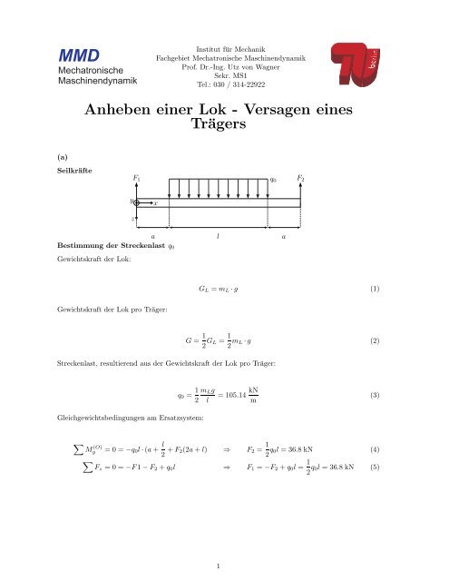
MMDMechatronischeMaschinendynamikInstitut für MechanikFachgebiet Mechatronische MaschinendynamikProf. Dr.-Ing. Utz von WagnerSekr. MS1Tel.: 030 / 314-22922Anheben einer Lok - Versagen einesTrägers(a)SeilkräfteF 1 q 0 F 2yxzaBestimmung der Streckenlast q 0Gewichtskraft der Lok:laG L = m L · g (1)Gewichtskraft der Lok pro Träger:G = 1 2 G L = 1 2 m L · g (2)Streckenlast, resultierend aus der Gewichtskraft der Lok pro Träger:q 0 = 1 m L g= 105.14 kN 2 l m(3)Gleichgewichtsbedingungen am Ersatzsystem:∑M(O)y = 0 = −q 0 l · (a + l 2 + F 2(2a + l) ⇒ F 2 = 1 2 q 0l = 36.8 kN (4)∑Fz = 0 = −F1 − F 2 + q 0 l ⇒ F 1 = −F 2 + q 0 l = 1 2 q 0l = 36.8 kN (5)1

(b)SchnittlastenverläufeDas Ersatzsystem wird in 3 Bereiche unterteilt:Bereich I (0 < x ≤ a)F 1M 1 (x)yxS 1N 1 (x)Q 1 (x)zx∑Fx = 0 = N 1 (x) (6)∑Fz = 0 = Q 1 (x) − F 1 ⇒ Q 1 (x) = F 1 = 1 2 q 0l (7)∑M(S 1)y = 0 = M 1 (x) − F 1 x ⇒ M 1 (x) = F 1 x = 1 2 q 0lx (8)Bereich II (a < x ≤ a + l)F 1q 0q 0 (x − a)M 2 (x)yxS 2N 2 (x)zx−a2Q 2 (x)ax − a∑Fx = 0 = N 2 (x) (9)∑Fz = 0 = Q 2 (x) − F1 + q 0 (x − a) ⇒ Q 2 (x) = 1 2 q 0l − q 0 (x − a) (10)∑M(S 2)y= 0 = M 2 (x) − F 1 x + q 0 (x − a) x − a2⇒ M 2 (x) = 1 2 q 0lx − q 02 (x − a)2 (11)2

Bereich III (a + l < x ≤ 2a + l)F 2M 3 (x)yxN 3 (x)S 3zxQ 3 (x)l + 2a∑Fx = 0 = N 3 (x) (12)∑Fz = 0 = −Q 3 (x) − F 2 ⇒ Q 3 (x) = − 1 2 q 0l (13)∑M(S 3)y = 0 = −M 3 (x) + F 2 (l + 2a − x) ⇒ M 3 (x) = 1 2 q 0l(l + 2a − x) (14)Grafische Darstellung der SchnittlastenverläufeBestimmung der Querkraft an den ausgezeichneten Punkten:Q 1 (x = 0) = 1 2 q 0l Q 1 (x = a) = 1 2 q 0l (15)Q 2 (x = a) = 1 2 q 0l Q 2 (x = a + l) = − 1 2 q 0l (16)Q 3 (x = a + l) = − 1 2 q 0l Q 3 (x = 2a + l) = − 1 2 q 0l (17)Bestimmung des Biegemoments an den ausgezeichneten Punkten:M 1 (x = 0) = 0 M 1 (x = a) = 1 2 q 0la (18)M 2 (x = a) = 1 2 q 0la M 2 (x = a + l) = 1 2 q 0la (19)M 3 (x = a + l) = 1 2 q 0la M 3 (x = 2a + l) = 0 (20)Maximalwert des Biegemoments ⇔ dM2(x)dx= M ′ 2 (x) ! = 0:⇒ M ′ 2 (x) = Q 2(x) ! = 0 ⇒12 q 0l − q 0 (x max − a) = 0 ⇒ x max = 1 2 l + a (21)⇒ M 2 (x max ) = q 0l 28 + q 0la= q ( )0l l2 2 4 + a(22)3

3020Q(x) in kN100.250.50.7511.251.5x in m−10−20−3025I II III20M(x) in kNm151050.250.50.7511.251.5x in m4

(c)Maximale NormalspannungFür die maximale Normalspannung gilt:Profil 1σ max = M bmaxz max = M bmax(23)I yy W bhyzIn der angegebenen Quelle findet man für h = 0.240 m, dass W b = W y1 = 3.00 ·10 −4 m 3 ist. Dasmaximale Biegemoment wurde in (b) bestimmt:⇒M bmax = M 2 (x = 1 2 l + a) = q 0l2( ) l4 + a = 24.823 kNm (24)⇒σ max = M bmax1W b= 8.2743 ·10 7 N m 2 (25)Profil 2hyzFür das um 90 ◦ gedrehte Profil findet man dass W b = W y2 = 3.96 ·10 −5 m 3 ist. Mit M bmax =24.823 kNm folgt:⇒σ max2 = M bmaxW b= 6.26843 ·10 8 N m 2 (26)(d)Vergleich der berechneten mit den zulässigen NormalspannungenMaximal zulässige Normalspannung für ST-37 bei ruhender Beanspruchung: σ zul = 1.1 ·10 8 N m 2Profil 1: σ max1 < σ zul ⇒ Träger hätte der Belastung stand gehaltenProfil 2: σ max2 > σ zul ⇒ Träger wurde plastisch deformiert5

(e)ClearRemove[w1,w2,w3,emodul,iy,F]emodul=210*10^9;m=7500;g=9.81;l=.7;a=.5;q0=m*g/l;iy=3600/10^(8);F=1/2*m*g;(*q(x)*)(*Q(x)*)(*M(x)*)(*w(x)*)(*k=DSolve[{w1’’’’[x]\[Equal]0,w1[0]\[Equal]0,w1’’[0]\[Equal]0,w1’’’[0]\[Equal]-F,w2’’’’[x]\[Equal]q0,w2[a]\[Equal]w1[a],w2’[a]\[Equal]w1’[a],w2’’[a]\[Equal]w1’’[a],w3’’’’[x]\[Equal]0,w3[a+l]\[Equal]w2[a+l],w3’[a+l]\[Equal]w2’[a+l],w3[2*a+l]\[Equal]0,w3’’[2*a+l]\[Equal]0,w3’’’[2*a+l]\[Equal]F/(EE*i)},{w1,w2,w3},x]*)(*Berechnung der Biegelinieerste Zeile: die vierten ableitungen der DGLzweite Zeile: Randbed. linker Rand (Biegung, Moment)dritte Zeile: Übergangsbed.bei x=a (Biegung, Winkel, Moment, Querkraft)vierte Zeile: Übergangsbed.bei x=a+l (Biegung, Winkel, Moment, Querkraft)fünfte Zeile: Randbed. rechter Rand (Biegung, Moment)*)k=DSolve[{w1’’’’[x]\[Equal]0,w2’’’’[x]\[Equal]q0/(emodul*iy),w3’’’’[x]\[Equal]0,w1[0]\[Equal]0,w1’’[0]\[Equal]0,w2[a]\[Equal]w1[a],w2’[a]\[Equal]w1’[a],w2’’[a]\[Equal]w1’’[a],w2’’’[a]\[Equal]w1’’’[a],w3[a+l]\[Equal]w2[a+l],w3’[a+l]\[Equal]w2’[a+l],w3’’[a+l]\[Equal]w2’’[a+l],w3’’’[a+l]\[Equal]w2’’’[a+l],w3[2*a+l]\[Equal]0,w3’’[2*a+l]\[Equal]0},{w1,w2,w3},x]w1[x_]=k\[LeftDoubleBracket]1,1,2,2\[RightDoubleBracket]w2[x_]=k\[LeftDoubleBracket]1,2,2,2\[RightDoubleBracket]w3[x_]=k\[LeftDoubleBracket]1,3,2,2\[RightDoubleBracket](*Plot[w1[x],{x,0,a}]Plot[w2[x],{x,a,a+l}]Plot[w3[x],{x,a+l,2*a+l}]*)(*Plotten des Biegemomentes*)6

moment1:=Plot[-w1’’[x]*(emodul*iy),{x,0,a},DisplayFunction\[Rule]Identity,PlotStyle\[Rule]{Thickness[0.001]},TextStyle\[Rule]{FontSize\[Rule]20}];moment2:=Plot[-w2’’[x]*(emodul*iy),{x,a,a+l},DisplayFunction\[Rule]Identity];moment3:=Plot[-w3’’[x]*(emodul*iy),{x,a+l,2*a+l},DisplayFunction\[Rule]Identity]Show[moment1,moment2,moment3,DisplayFunction\[Rule]$DisplayFunction,AxesLabel\[Rule]{"x","M(x)"}];(*Plotten der Querkraft*)quer1:=Plot[-w1’’’[x]*(emodul*iy),{x,0,a},DisplayFunction\[Rule]Identity,PlotStyle\[Rule]{Thickness[0.001]},TextStyle\[Rule]{FontSize\[Rule]20}];quer2:=Plot[-w2’’’[x]*(emodul*iy),{x,a,a+l},DisplayFunction\[Rule]Identity];quer3:=Plot[-w3’’’[x]*(emodul*iy),{x,a+l,2*a+l},DisplayFunction\[Rule]Identity]Show[quer1,quer2,quer3,DisplayFunction\[Rule]$DisplayFunction,AxesLabel\[Rule]{"x","Q(x)"}];(*Plotten der Biegelinie*)biege1:=Plot[-w1[x],{x,0,a},DisplayFunction\[Rule]Identity,PlotStyle\[Rule]{Thickness[0.001]},TextStyle\[Rule]{FontSize\[Rule]20}];biege2:=Plot[-w2[x],{x,a,a+l},DisplayFunction\[Rule]Identity];biege3:=Plot[-w3[x],{x,a+l,2*a+l},DisplayFunction\[Rule]Identity]Show[biege1,biege2,biege3,DisplayFunction\[Rule]$DisplayFunction,AxesLabel\[Rule]{"x","-w(x)"}];(*Durchbiegung im mm an der Stelle a+l/2*)w2[a+l/2]*1000(*Querkräfte an Rändern und mitte*)w1’’’[0]w3’’’[2+a+l]w2’’’[a+l/2] (*sollte Null sein*)x in m0.25 0.5 0.75 1 1.25 1.50.0002w(x)0.00040.00060.00087