- Page 2 and 3:
Decision Analysis for Management Ju
- Page 5 and 6:
Decision Analysis for Management Ju
- Page 7:
To Mary and Josephine, Jamie, Jerom
- Page 10 and 11:
viii Contents Chapter 16 The analyt
- Page 12 and 13:
x Foreword real problems, and it is
- Page 14 and 15:
xii Preface accountancy, where rece
- Page 17 and 18:
1 Introduction Complex decisions Im
- Page 19 and 20:
The role of decision analysis 3 you
- Page 21 and 22:
Applications of decision analysis 5
- Page 23 and 24:
Applications of decision analysis 7
- Page 25 and 26:
Applications of decision analysis 9
- Page 27 and 28:
Overview of the book 11 and profit.
- Page 29:
References 13 8. Walls, M. R., Mora
- Page 32 and 33:
16 How people make decisions involv
- Page 34 and 35:
18 How people make decisions involv
- Page 36 and 37:
20 How people make decisions involv
- Page 38 and 39:
22 How people make decisions involv
- Page 40 and 41:
24 How people make decisions involv
- Page 42 and 43:
26 How people make decisions involv
- Page 44 and 45:
28 Decisions involving multiple obj
- Page 46 and 47:
30 Decisions involving multiple obj
- Page 48 and 49:
32 Decisions involving multiple obj
- Page 50 and 51:
34 Decisions involving multiple obj
- Page 52 and 53:
36 Decisions involving multiple obj
- Page 54 and 55:
38 Decisions involving multiple obj
- Page 56 and 57:
40 Decisions involving multiple obj
- Page 58 and 59:
42 Decisions involving multiple obj
- Page 60 and 61:
44 Decisions involving multiple obj
- Page 62 and 63:
46 Decisions involving multiple obj
- Page 64 and 65:
48 Decisions involving multiple obj
- Page 66 and 67:
50 Decisions involving multiple obj
- Page 68 and 69:
52 Decisions involving multiple obj
- Page 70 and 71:
54 Decisions involving multiple obj
- Page 72 and 73:
56 Decisions involving multiple obj
- Page 74 and 75: 58 Decisions involving multiple obj
- Page 76 and 77: 60 Decisions involving multiple obj
- Page 78 and 79: 62 Decisions involving multiple obj
- Page 80 and 81: 64 Decisions involving multiple obj
- Page 82 and 83: 66 Decisions involving multiple obj
- Page 84 and 85: 68 Decisions involving multiple obj
- Page 86 and 87: 70 Decisions involving multiple obj
- Page 88 and 89: 72 Introduction to probability Beca
- Page 90 and 91: 74 Introduction to probability prac
- Page 92 and 93: 76 Introduction to probability we w
- Page 94 and 95: 78 Introduction to probability whet
- Page 96 and 97: 80 Introduction to probability give
- Page 98 and 99: 82 Introduction to probability prob
- Page 100 and 101: 84 Introduction to probability deci
- Page 102 and 103: 86 Introduction to probability that
- Page 104 and 105: 88 Introduction to probability inte
- Page 106 and 107: 90 Introduction to probability subj
- Page 108 and 109: 92 Introduction to probability (5)
- Page 110 and 111: 94 Introduction to probability (a)
- Page 112 and 113: 96 Decision making under uncertaint
- Page 114 and 115: 98 Decision making under uncertaint
- Page 116 and 117: 100 Decision making under uncertain
- Page 118 and 119: 102 Decision making under uncertain
- Page 120 and 121: 104 Decision making under uncertain
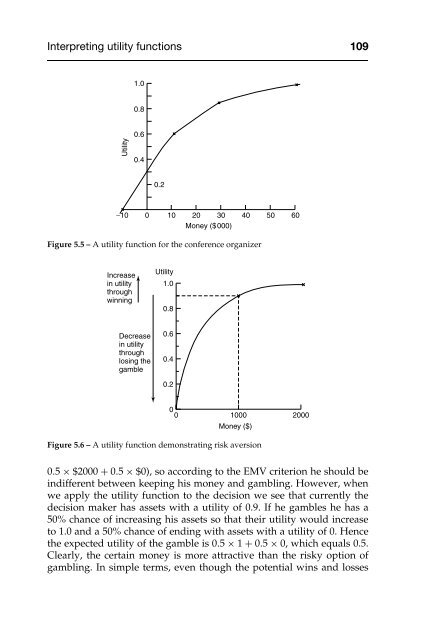
- Page 122 and 123: 106 Decision making under uncertain
- Page 126 and 127: 110 Decision making under uncertain
- Page 128 and 129: 112 Decision making under uncertain
- Page 130 and 131: 114 Decision making under uncertain
- Page 132 and 133: 116 Decision making under uncertain
- Page 134 and 135: 118 Decision making under uncertain
- Page 136 and 137: 120 Decision making under uncertain
- Page 138 and 139: 122 Decision making under uncertain
- Page 140 and 141: 124 Decision making under uncertain
- Page 142 and 143: 126 Decision making under uncertain
- Page 144 and 145: 128 Decision making under uncertain
- Page 146 and 147: 130 Decision making under uncertain
- Page 148 and 149: 132 Decision making under uncertain
- Page 150 and 151: 134 Decision making under uncertain
- Page 152 and 153: 136 Decision making under uncertain
- Page 154 and 155: 138 Decision making under uncertain
- Page 156 and 157: 140 Decision making under uncertain
- Page 159 and 160: 6 Decision trees and influence diag
- Page 161 and 162: Constructing a decision tree 145 be
- Page 163 and 164: Determining the optimal policy 147
- Page 165 and 166: Decision trees and utility 149 succ
- Page 167 and 168: Decision trees involving continuous
- Page 169 and 170: Practical applications of decision
- Page 171 and 172: Assessment of decision structure 15
- Page 173 and 174: Assessment of decision structure 15
- Page 175 and 176:
Eliciting decision tree representat
- Page 177 and 178:
Eliciting decision tree representat
- Page 179 and 180:
Summary 163 where the resulting dec
- Page 181 and 182:
Exercises 165 other elements of the
- Page 183 and 184:
Exercises 167 (b) Assuming that Wes
- Page 185 and 186:
Exercises 169 is not hired, given t
- Page 187 and 188:
Exercises 171 failing to meet the p
- Page 189 and 190:
Exercises 173 why it was rational f
- Page 191 and 192:
Exercises 175 (11) In the Eagle Mou
- Page 193 and 194:
References 177 ABC Chemicals are pl
- Page 195 and 196:
7 Applying simulation to decision p
- Page 197 and 198:
Monte Carlo simulation 181 Of cours
- Page 199 and 200:
Monte Carlo simulation 183 Table 7.
- Page 201 and 202:
Applying simulation to a decision p
- Page 203 and 204:
Applying simulation to a decision p
- Page 205 and 206:
Applying simulation to a decision p
- Page 207 and 208:
Applying simulation to a decision p
- Page 209 and 210:
Applying simulation to a decision p
- Page 211 and 212:
Applying simulation to a decision p
- Page 213 and 214:
Applying simulation to investment d
- Page 215 and 216:
Applying simulation to investment d
- Page 217 and 218:
Applying simulation to investment d
- Page 219 and 220:
Applying simulation to investment d
- Page 221 and 222:
Summary 205 Hull 10 ), some of them
- Page 223 and 224:
Exercises 207 (c) Use your simulati
- Page 225 and 226:
Exercises 209 For each factor the f
- Page 227 and 228:
Exercises 211 (b) Suppose that your
- Page 229:
References 213 6 million Therefore
- Page 232 and 233:
216 Revising judgments in the light
- Page 234 and 235:
218 Revising judgments in the light
- Page 236 and 237:
220 Revising judgments in the light
- Page 238 and 239:
222 Revising judgments in the light
- Page 240 and 241:
224 Revising judgments in the light
- Page 242 and 243:
226 Revising judgments in the light
- Page 244 and 245:
228 Revising judgments in the light
- Page 246 and 247:
230 Revising judgments in the light
- Page 248 and 249:
232 Revising judgments in the light
- Page 250 and 251:
234 Revising judgments in the light
- Page 252 and 253:
236 Revising judgments in the light
- Page 254 and 255:
238 Revising judgments in the light
- Page 256 and 257:
240 Revising judgments in the light
- Page 258 and 259:
242 Revising judgments in the light
- Page 260 and 261:
244 Revising judgments in the light
- Page 263 and 264:
9 Biases in probability assessment
- Page 265 and 266:
Introduction 249 of people watching
- Page 267 and 268:
The availability heuristic 251 make
- Page 269 and 270:
The representativeness heuristic 25
- Page 271 and 272:
The representativeness heuristic 25
- Page 273 and 274:
The representativeness heuristic 25
- Page 275 and 276:
The anchoring and adjustment heuris
- Page 277 and 278:
The anchoring and adjustment heuris
- Page 279 and 280:
Other judgmental biases 263 Other j
- Page 281 and 282:
Is human probability judgment reall
- Page 283 and 284:
Is human probability judgment reall
- Page 285 and 286:
Is human probability judgment reall
- Page 287 and 288:
Exercises 271 Did you receive timel
- Page 289 and 290:
References 273 have been taken from
- Page 291 and 292:
References 275 18. Hamilton, D. L.
- Page 293 and 294:
10 Methods for eliciting probabilit
- Page 295 and 296:
Preparing for probability assessmen
- Page 297 and 298:
Preparing for probability assessmen
- Page 299 and 300:
Preparing for probability assessmen
- Page 301 and 302:
Consistency and coherence checks 28
- Page 303 and 304:
Assessment of the validity of proba
- Page 305 and 306:
Assessment of the validity of proba
- Page 307 and 308:
Assessing probabilities for very ra
- Page 309 and 310:
Exercises 293 Odds in favor of even
- Page 311:
References 295 13. Wright, G. and W
- Page 314 and 315:
298 Risk and uncertainty management
- Page 316 and 317:
300 Risk and uncertainty management
- Page 318 and 319:
302 Risk and uncertainty management
- Page 320 and 321:
304 Risk and uncertainty management
- Page 322 and 323:
306 Risk and uncertainty management
- Page 324 and 325:
308 Risk and uncertainty management
- Page 326 and 327:
310 Decisions involving groups of i
- Page 328 and 329:
312 Decisions involving groups of i
- Page 330 and 331:
314 Decisions involving groups of i
- Page 332 and 333:
316 Decisions involving groups of i
- Page 334 and 335:
318 Decisions involving groups of i
- Page 336 and 337:
320 Decisions involving groups of i
- Page 338 and 339:
322 Decisions involving groups of i
- Page 340 and 341:
324 Decisions involving groups of i
- Page 342 and 343:
326 Decisions involving groups of i
- Page 344 and 345:
328 Decisions involving groups of i
- Page 346 and 347:
330 Resource allocation and negotia
- Page 348 and 349:
332 Resource allocation and negotia
- Page 350 and 351:
334 Resource allocation and negotia
- Page 352 and 353:
336 Resource allocation and negotia
- Page 354 and 355:
338 Resource allocation and negotia
- Page 356 and 357:
340 Resource allocation and negotia
- Page 358 and 359:
342 Resource allocation and negotia
- Page 360 and 361:
344 Resource allocation and negotia
- Page 362 and 363:
346 Resource allocation and negotia
- Page 364 and 365:
348 Resource allocation and negotia
- Page 366 and 367:
350 Resource allocation and negotia
- Page 368 and 369:
352 Resource allocation and negotia
- Page 371 and 372:
14 Decision framing and cognitive i
- Page 373 and 374:
How people frame decisions 357 Figu
- Page 375 and 376:
Imposing imaginary constraints and
- Page 377 and 378:
Inertia in strategic decision makin
- Page 379 and 380:
Studies in the psychological labora
- Page 381 and 382:
Studies in the psychological labora
- Page 383 and 384:
Studies in the psychological labora
- Page 385 and 386:
Overcoming inertia? 369 it is diffi
- Page 387 and 388:
Studies in the psychological labora
- Page 389 and 390:
Discussion questions 373 frame anal
- Page 391 and 392:
References 375 References 1. Luchin
- Page 393 and 394:
15 Scenario planning: an alternativ
- Page 395 and 396:
Introduction 379 documented in Chap
- Page 397 and 398:
Scenario construction: the extreme-
- Page 399 and 400:
Using scenarios in decision making
- Page 401 and 402:
Using scenarios in decision making
- Page 403 and 404:
Scenario construction: the driving
- Page 405 and 406:
Scenario construction: the driving
- Page 407 and 408:
Scenario construction: the driving
- Page 409 and 410:
Case study of a scenario interventi
- Page 411 and 412:
Case study of a scenario interventi
- Page 413 and 414:
Case study of a scenario interventi
- Page 415 and 416:
Case study of a scenario interventi
- Page 417 and 418:
Table 15.1 - The components of the
- Page 419 and 420:
Illustrative case study 403 (b) Att
- Page 421 and 422:
Illustrative case study 405 Stage 4
- Page 423 and 424:
Illustrative case study 407 importa
- Page 425 and 426:
Conclusion 409 combinations. Often
- Page 427:
References 411 2. Van der Heijden,
- Page 430 and 431:
414 The analytic hierarchy process
- Page 432 and 433:
416 The analytic hierarchy process
- Page 434 and 435:
418 The analytic hierarchy process
- Page 436 and 437:
420 The analytic hierarchy process
- Page 438 and 439:
422 The analytic hierarchy process
- Page 440 and 441:
424 The analytic hierarchy process
- Page 443 and 444:
17 Alternative decision-support sys
- Page 445 and 446:
Expert systems 429 generally agreed
- Page 447 and 448:
Expert systems 431 that knowledge e
- Page 449 and 450:
Expert systems 433 (1) That the sub
- Page 451 and 452:
Expert systems 435 information syst
- Page 453 and 454:
Expert systems 437 to focus on ‘t
- Page 455 and 456:
Expert systems 439 On the basis of
- Page 457 and 458:
Is there any intention/expectation
- Page 459 and 460:
Expert systems 443 described above
- Page 461 and 462:
Expert systems 445 body of knowledg
- Page 463 and 464:
Statistical models of judgment 447
- Page 465 and 466:
Statistical models of judgment 449
- Page 467 and 468:
Statistical models of judgment 451
- Page 469 and 470:
Comparisons 453 ‘broken leg’ cu
- Page 471 and 472:
Some final words of advice 455 Ques
- Page 473 and 474:
Some final words of advice 457 of t
- Page 475 and 476:
References 459 Table 17.1 - Summary
- Page 477 and 478:
References 461 20. Eisenhart, J. (1
- Page 479 and 480:
Chapter 3 Suggested answers to sele
- Page 481 and 482:
Suggested answers to selected quest
- Page 483 and 484:
Suggested answers to selected quest
- Page 485:
Suggested answers to selected quest
- Page 488 and 489:
472 Index Brown, C.E. 446 Brown, S.
- Page 490 and 491:
474 Index HIVIEW 58 Hodgkinson, G.P
- Page 492 and 493:
476 Index scenario intervention cas