Unified Database Theory - ODBMS

ABSTRACT
The paper provides a common mathematical database theory
that unifies relational databases, data warehouse models and
object-oriented database models. It is based on long experiences
reflected in human language models and database system
development. This is a short version of the theory. The
complete version can be requested at reinhard.karge@runsoftware.com.
The paper discusses a state model as the base for storing data in
a database. This includes specific ways of collecting states in
instances and instance collections as well as ordering states in
classes by means of classifications. Thus, database models can
be described on four different levels according to the degree of
order in the database.
The paper investigates how far principles of presenting
knowledge in human language can be used as basic rules for
building database systems. It shows a way to formalize
knowledge presentation in human language and how human
language principles as ordering facts, referring to behaviour and
causalities can be used for building database models.
Theoretical and practical benefits of human language oriented
DBMS (database management systems) are demonstrated. The
paper is based on practical experiences in developing database
management systems (mainly the object-oriented DBMS
ODABA) with the goal of supporting human language oriented
knowledge presentations.
Keywords: database, modelling techniques, human language
model, set algebra, knowledge presentation
INTRODUCTION
One possible approach is to define modeling rules that follow
principles of knowledge presentation in human language.
Human language presentations differ between presenting
concepts and facts, even though this is not obvious. Concepts
describe the way facts are represented, i.e. one cannot
communicate about facts without having the same concepts in
mind. For defining concepts, those are explained usually as
facts referring to concepts about concepts. Such concepts about
concepts we will call human language model (HLM).
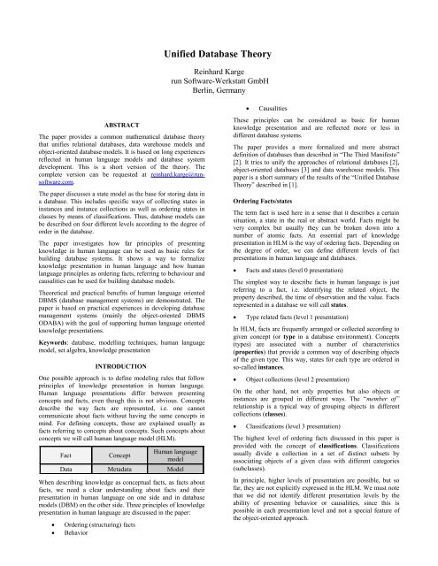
Fact Concept
Unified Database Theory
Reinhard Karge
run Software-Werkstatt GmbH
Berlin, Germany
Human language
model
Data Metadata Model
When describing knowledge as conceptual facts, as facts about
facts, we need a clear understanding about facts and their
presentation in human language on one side and in database
models (DBM) on the other side. Three principles of knowledge
presentation in human language are discussed in the paper:
Ordering (structuring) facts
Behavior
Causalities
These principles can be considered as basic for human
knowledge presentation and are reflected more or less in
different database systems.
The paper provides a more formalized and more abstract
definition of databases than described in “The Third Manifesto”
[2]. It tries to unify the approaches of relational databases [2],
object-oriented databases [3] and data warehouse models. This
paper is a short summary of the results of the “Unified Database
Theory” described in [1].
Ordering Facts/states
The term fact is used here in a sense that it describes a certain
situation, a state in the real or abstract world. Facts might be
very complex but usually they can be broken down into a
number of atomic facts. An essential part of knowledge
presentation in HLM is the way of ordering facts. Depending on
the degree of order, we can define different levels of fact
presentations in human language and databases.
Facts and states (level 0 presentation)
The simplest way to describe facts in human language is just
referring to a fact, i.e. identifying the related object, the
property described, the time of observation and the value. Facts
represented in a database we will call states.
Type related facts (level 1 presentation)
In HLM, facts are frequently arranged or collected according to
given concept (or type in a database environment). Concepts
(types) are associated with a number of characteristics
(properties) that provide a common way of describing objects
of the given type. This way, states for each type are ordered in
so-called instances.
Object collections (level 2 presentation)
On the other hand, not only properties but also objects or
instances are grouped in different ways. The “member of”
relationship is a typical way of grouping objects in different
collections (classes).
Classifications (level 3 presentation)
The highest level of ordering facts discussed in this paper is
provided with the concept of classifications. Classifications
usually divide a collection in a set of distinct subsets by
associating objects of a given class with different categories
(subclasses).
In principle, higher levels of presentation are possible, but so
far, they are not explicitly expressed in the HLM. We must note
that we did not identify different presentation levels by the
ability of presenting behavior or causalities, since this is
possible in each presentation level and not a special feature of
the object-oriented approach.

Rule/behavior and operation/functions
Besides simply presenting facts, human language is able to
describe abstract rules about relations or dependencies between
facts or the way facts will change (behavior). On the other hand,
we can combine different facts to create derived facts by means
of rules, or we can define rules for many other purposes. In a
database context, we will refer to such rules as operation.
Behavior is usually not described for a specific process but as
an abstraction of changes or dependencies. Thus, describing
behavior is another way of expressing knowledge in HLM or in
databases. The definition of operations is not bound to a
specific presentation level. However, the complexity of rules
that can be expressed on different levels is different.
Causality and event/reaction
Another basic principle in HLM is the presentation of
causalities, i.e. the relation between cause (or reason) and its
consequences. A cause is a certain constellation of facts that
causes a typical reaction in the world. Sometimes, a special
behavior is considered as cause, but this is only one specific
way to create a constellation of facts considered as cause.
Thus, in the paper we will consider relevant state transitions as
cause and the consequence as resulting behavior (which might
cause other state transitions). On the database level causes are
presented as event and the consequence as reaction.
Cause and consequence are reflected in HLM as facts but also
as abstractions. Thus, causalities are described as specific
constellations on the data level but also as abstract causalities
on the conceptual level.
BASIC STATE MODEL
The basic state model describes principles and basic
assumptions made for describing abstract database models. The
basic state model considers how facts can be presented as states
of objects in a database. It is based on the assumption that each
fact is associated with an object, i.e. that a fact describes a
property or attribute of an elementary or abstract object.
Here, an object is considered as an abstract term, which
includes elementary (real world) objects as well as abstract
objects (ideas, concepts …), i.e. everything that may carry
attributes or properties is considered as an object.
Atomic State
The state of an elementary or abstract object is defined in terms
of different properties as quality, attributes or relations. For
simplicity reasons we can assume:
A1: An atomic state describes the relation between an
identifiable object (o) and a property (p) with a property value
(v) at a given point in time (t).
S = { s = (o,t,p,v) : oO, pP, vVp , tTI } (1a)
Here, O is the set of all objects taken into consideration, P is a
set of defined properties and TI is a set of relevant time values.
Vp is the property value domain. Theoretically, the properties
value domain may present any type of symbols or all possible
bit strings (in a database environment), but practically more
specific property domains can be defined on the conceptual
level.
A2: Two states are considered as identical when referring to the
same object, property and time value:
s1,s2 S o1 = o2 p1 = p2 t1 = t2 s1 = s2
Than we can assume:
s1,s2 S : s1 = s2 v1 = v2
(1b)
(1c)
This means that a state can have exactly one value. Thus, the
state definition introduces three identifying components for a
state as (o,t,p), while the value is a quantitative or qualitative
component in the state. Object and time can be considered
usually as given real world phenomena, but there are also
conceptual objects and time values. The property is a pure
human concept. Practically, the whole HLM is based on the
assumption of common concepts. The decision, whether two
properties are identical, is a conceptual decision (a definition)
that allows grouping states by properties.
There is obviously no dependency between object and time
dimension of a state. Properties as human concepts, however,
might change over time. We will assume that conceptual
changes result in new properties. This is a critical assumption,
which should be solved in future. Sometimes, properties appear
as dependent on the carrying object. There are many reasons for
an object not having a state for a certain property. To resolve
this complication we will assume:
A3: There exists an empty value in each value domain Vp.
The specific behaviour of the empty value in operations is part
of the definition of the operation.
When the state value for an object o and the property p at time t
is for “non-applicable” properties, we can combine each
property with each object at any time point. Thus, we can
assume:
A4: Object, time and property are independent state
dimensions.
Defining the property as independent dimension, we can also
consider the value domain Vp as independent on object and
time, i.e. changing the value domain for a property results in or
is the consequence of defining a new property.
D01: An abstract state a = (o,t,p) is defined as state without
value. The set of all possible abstract states, the abstract state
set A is defined as product set of the state dimensions:
A = O x P x TI (1d)
O, P and TI are considered as object, property and time domain
of a database. Abstract states allow describing states on a
conceptual level. Usually, only a subset of abstract states is
stored as state in the database but abstract state sets are the base
for describing schemata, operations and causalities on the
conceptual level. Considering S as the set of states in a
database, the set of abstract states stored in S is defined as:
A(S) = { a : a=A(s) s S } (1e)
Complex States
A complex state is a collection of states. Complex states do not
exist by nature but are rather an expression of human
knowledge. Grouping states into complex states is the basic
method for creating high level (Р1, Р2, Р3) database models.
Besides, complex states allow expressing dependencies or other
types of connections between facts and play an important rule
for describing operations and causalities.
In the following chapters, we will refer to finite sets of objects,
time values, properties, states, abstract states etc with n
elements as vectors:

Xn = n
i1 xi = (x1, …, xn) (1f)
Here X stands for O, P, T, S, A etc. X defines a vector with a
finite but undefined number of elements.
D02: A complex state Sn is a finite set of distinct states in S:
Sn S : A(si) A(sj) i, j : 1 i,j n i j (1g)
The rules for grouping states to complex states are often
described by means of abstract states in a state schema.
State Schema
There are many ways in HML of defining rules for building
complex states according to a given schema. Usually, a schema
defines a way of grouping states in a complex state by means of
abstract states.
D03: A state schema is a set of abstract states a complex state is
based on.
A(Sn) = An : ai = A(si) (2a)
Since states in a complex state are distinct, abstract states in
schema are distinct as well. Supposing, that abstract states,
which are not stored in the database, will result in an empty
state value, we will get exactly one complex state Sn when
applying a state schema on a state set S (database):
An(S) = Sn
(2b)
Thus, a state schema is a conceptual definition on the one hand
and an access operation on the other hand.
The value domain for each state in a complex state depends
only on the property. Hence, the value domain for a state
schema can be defined as:
V(An) = V(Pn) =
n
i 1
V p (2c)
i
D04: A state schema is called orthogonal when it can be
divided in independent time, object and property dimensions:
An = Oi x Tj x Pk : n = i*j*k (2d)
Oi is called object dimension, Tj time dimension and Pk
property dimension. The state schema is called (Oi, Tj, Pk)
schema.
Since abstract states in a complex state schema are distinct,
objects, time values and properties of an orthogonal schema
must be distinct as well.
Semi-orthogonal schemata
An orthogonal schema requires a three dimensional model for
describing data. Several data models, however, support two
dimensional models, only, that are based on semi-orthogonal
schemata.
D05: A state schema is called semi-orthogonal when it can be
divided in independent object/time and property, object and
property/time or object/property and time dimension as:
An = OTm x Pk : OTm Oi x Tj
An = OPm x Tj : OPm Oi x Pk
An = PTm x Oi : PTm Tj x Pk
(2e)
(2f)
(2g)
This describes all possible semi-orthogonal schemata, even
though the (OTm, Pk) schema is the typical case while the
(OPm, Tj) schema is rarely used.
Schema Family
While a schema describes the intention of a state set, the schema
family describes the extension of a state set.
D06: A schema family SF describes a set of semi-orthogonal
schemata (I,E) with a constant vector I.
I is called the intentional dimension of the schema family, while
E is the extensional dimension. In principle, any of the two
dimensions of a semi-orthogonal schema might become the
intentional dimension, but usually the dimension with the
property component is considered as intentional dimension.
Hence, we will consider mainly the O, T and OT dimension as
extensional dimensions.
We will refer to a finite set of vectors as:
X
{ X : X X } (3a)
X n describes a subset of X containing n vectors. Now, we
can define an object extension as O . Since the number of
objects in a database is finite, O is finite as well. The same
way, we can define a set of time vectors. T . The number of
time values is not finite in reality. For a database, however, we
can assume that there is a minimum distance between the time
points of two facts, i.e.
A5: There exists a minimum time interval t, which is the
minimum measure distance between two observations in the
database.
t TI t > 0 : t1 – t2 > t s1,s2 S t1 > t2 (3b)
Now, the time domain TI for a database becomes finite andT is
finite as well. At least OT defines a set of property/time
vectors. Since it does not make sense considering extensions on
property vectors, we will consider only object, time and
object/time extensions.
D7: A regular schema family is a schema family with a distinct
set of states:
Aa, Ab SF Aa Ab Aa Ab = (3c)
Since the property dimension is constant, elements in the
object/time dimension for a regular schema family are distinct.
Then, we can show, that:
S1: Each regular schema family is equivalent to a semiorthogonal
schema with the same intentional dimension.
S2: Each semi-orthogonal schema, which is not an (o, t, Pk)
schema, is equivalent to a regular schema family.
D8: A finite set of schemata SFn where the schemata are based
on each other, is called grouping schema.
SFi SF i > 1 SFi+1 = SF(SFi) (3d)
There might be any number of schema families for a schema as
well as any number of sub-schemata. Unfortunately, schema
families may run into recursion. On the other hand, the
grouping function for a schema family does not depend on the
intentional dimension, i.e. that the grouping schema is defined
by the extensional dimension, only.
D09: A type schema is a schema that is equivalent to a regular (
OT , Pk), (O , TPk) or (T , OPk) schema family or to an (o, t,
Pk) schema.

A type schema defines an intentional component of a schema
family, which is fixed in dimension and thus, conceptually
predefined, and an extensional component, which is defined as
grouping schema. Now, we can show, that:
S3: Each type schema can be divided into a finite number of
orthogonal (O, T, Pk) type schemata.
SF = n
i1 (O i, T i, Pki) (O , T , P ) (3e)
Several statements on the following pages are restricted to
orthogonal type schemata. This is, however, more a theoretical
restriction, since most known schemata are orthogonal type
schemata or can be divided into a number of orthogonal
schemata.
SCHEMA COMPONENT
In an orthogonal type schema the intentional component Pk is
called type. The extensional components O and T are
described as object schema and time schema, which are
grouping schemata for the object and time dimension.
Object schema
The conceptual part of an object schema is the definition of
object collections O for the sub-schemata and relations between
sub-schema and grouping objects. Conceptually an object
collection may express a grouping approach as well as a
collection of objects with well defined roles.
A6: In an object schema, each object collection is defined in the
context of exactly one object og, which is called the grouping
object for O.
Typical examples for object schemata are grouping hierarchies
or object frames (pre-defined sets of objects). Object schemata
can be expressed in three ways. Typically and well known are
object relations, where each grouping object is related to the
objects that it is grouping.
Og(t,p) = { (o, og) O x O } (3f)
Since collections may change over time, grouping relations are
time depending. The object relation may describe a 1:1, 1:N,
N:1 or M:N relation. This means practically, that both objects in
the relation could be considered as grouping object including
the case that an object group consists of only one object. Hence,
we can also define an inverse grouping relation Ig(Og(t,p)) for
each object relation with:
Ig(Og(t,p)) = { (og, o) : (o, og) Og(t,p) } (3g)
D10: A collection property is a property, where the value
domain is a set of object vectors:
sc = (o,t,pc,v) : V(pc) O
(3h)
Since there exists an inverse grouping function each collection
property has an inverse collection property that defines the
inverse collection of the object relation.
The third way is expressing an object schema by means of
membership states.
D11: The membership state for a given object collection O at a
certain time point t is defined as follows:
v = o O(t,p) : s = (o, t, p, v) Vp = {true,} (3i)
where O(t,p) is the object collection described by the
membership property p at time t.
As well as property collections membership states imply an
inverse membership property for each membership property.
S4: Presentations of grouping relations by means of
membership properties, object relations and collection
properties are equivalent.
Thus, it is only a matter of operations to be performed, which
one to choose. For access functions the collection properties are
most comfortable, while causalities are easier to describe by
means of membership properties. An object relation is the most
efficient way of storing membership states, since it does not
require an explicit inverse element.
Grouping is based on the assumption that there exists at least
one grouping object for each object collection (A6). Since
grouping objects can be grouped again etc, an object set O may
contain any number of grouping objects.
D12: An object grouping schema O is an object schema,
which defines exactly one generating object set for each object
in O:
o O E On O : o = G(On)
Objects in a grouping schema with o = G({o}) are called
elementary objects. Objects in a grouping schema, which are
not elementary, are called aggregated objects.
For a grouping schema, we can define the inverse grouping
function I as:
I(o) = On
which describes the ungrouping of objects.
D13: An object grouping schema O is called recursive, when
(3k)
In(O) OE : n = dim(O) (3l)
A non-recursive schema is called object hierarchy.
In a hierarchy, each object belongs to exactly one level, where
the level L(o) is the maximum number of possible ungroupings
for each object in I(o), until it ends up in an elementary object.
D14: An object hierarchy is called strict, when for all
aggregated objects in a hierarchy
o OA: L(oi) = L(o)-1 oi I(o) (3m)
D15: A object grouping schema is called distinct, when
oa,obOA : oa ob I(oa) I(ob) = (3n)
We can define the set of aggregated objects on level k in the
hierarchy as:
Lk(O) = { o OA : L(o) = k k > 0 } (3o)
D16: A strict object hierarchy is called complete, when for all
aggregated objects for each level in the hierarchy
k > 0 : I(Lk(O)) Lk-1(O) (3p)
Thus, in a complete hierarchy each higher level aggregates all
the objects on the next lower level.
D17: A complete and distinct object hierarchy is called
classification.
Considering aggregated objects as conceptual objects
(categories), they can be defined without any relationship to
elementary objects as conceptual hierarchies or classifications.
A conceptual object hierarchy may apply to any object
collection. In contrast to conceptual object hierarchies, ad hoc
hierarchies can be defined by defining a hierarchy of grouping

objects and associated generic membership properties. Ad hoc
classifications are more flexible, since categories correspond to
objects in this case, which are created on demand.
Each aggregated object in an object hierarchy defines a class of
elementary objects:
C(o) = Ik(o) : k = L(o) (3q)
When applying a conceptual classification on a set of
(elementary) objects, the conceptual classification will create
object classes. Thus, conceptual classifications are operations
that provide a set of distinct object classes on each level of the
hierarchy, when applying on a set of elementary objects.
For an object set many hierarchies can be defined, which share
at least the “total” level. In general, each level in an object
schema might have many sub-schemata and many parent
schemata. Thus, we can consider an extended object schema as
a family of hierarchies or classification, which is described as an
acyclic directed graph of hierarchy levels [1].
Component Schema
In many cases, an object schema can be described as orthogonal
schema. An orthogonal object schema can be expressed as
product of components:
n
O = O i
(3r)
i1
When any of the object components Oi in the schema is
described as family of object hierarchies O(i), we can define
separate aggregations for those object components. This makes
sense, only, when the grouping schema for each component
refers to the same set of elementary objects.
Time Schema
A time schema defines a rule for creating a set of time points or
time intervals T. In principle, a time schema follows the same
rules as an object schema. The difference is, that time represents
a continuum while object sets can be considered as discrete. On
the other hand, time has usually a known value domain, which
is not the case for objects. Thus, time schemata are usually
conceptually ones. Similar to object schemata we can define
hierarchies and classification for time schema [1].
Time schemata are very simple in many cases as being defined
for a fixed time value (interval or point) or presenting all
“current” states (time is always “now”). But there are more
complex time schemata and the interest in time schemata is
growing.
Type schema
Types in a type schema are used to order the properties of a
database schema according to basic concepts (types).
D18: A type defines the intentional dimension in a type
schema.
Thus, the type might be based on an (o,TPm) schema as well as
on an (t,OPm) schema. Since those schemata can be divided into
a finite number of (o,t,Pk) schemata, we will consider Pk types,
only.
T = Pk Pk P
(4a)
The set of all types T in a database schema is then defined as
subset of P . We can consider a schema as valid, when it does
not contain duplicate abstract states. Then it follows:
S5: A type schema is valid when the types defined in the sub
schemata are distinct.
T1,T2 T T1T2 T1 T2 = (4b)
We will use a combination of type and property name T.p to
identify a property. In many cases we refer to complex
properties based on a type again (e.g. address of residence).
Thus, complex properties can be associated with a type, while
the type for elementary properties is . Now we can introduce a
type function that returns a type for each property:
Ts = T(p) : p P Ts T (4c)
D19: A property with T(p) is called typed property.
Since T(p) is a type Ts we can refer to properties ps in Ts as
Ts.ps or T(p).ps or shortly as T.p.ps.replacing the type function
by the ‘dot operator’. Then we can define property paths as:
p = T.pn : pi+1 T(pi) : i = 1 … n-1 (4d)
Then T.pn defines the set of all property paths with length n.
We can consider each typed property as collection property,
which refers to a set of related objects. Then, T.p defines a
grouping function for typed properties, where any object of type
T groups the objects in the typed property p. It can be shown,
that
S6: Each typed property path T.pn defines a grouping hierarchy
of level n.
This means that each property path defines an ad hoc hierarchy
or classification. In contrast to conceptual grouping schemata,
ad hoc grouping schemata define the links, while the grouping
depends on the states stored in the database. Finally, it follows:
S6: Each property path defines a type schema.
pnP: SF(o,t,pn) = (O, t, Pk) (4e)
Since access operations as well as set and other operations are
based on schemata, property paths can be referred to in any
operation that is based on an appropriate type schema.
Applying a type on a database S at a certain time point will
result in a schema as:
T(t,S) = (O,T,Pk) (4f)
Thus, each type defines also an extension and can be considered
as grouping schema.
On the other hand, we can add an intentional aspect to any
classification, i.e. each class (grouping object) in a classification
becomes a type. In this case, each grouping class is the base
type for the grouped objects.
DATABASE MODELS
A general problem results from the fact, that the existence of
any object might be philosophically doubtful, but in human
reflections, objects do not exist at all, i.e. at least human
language is reflecting concepts, which are related to types rather
than to objects. Practically, the whole object-oriented approach
turns out to be a type-oriented one. Since the object concept is
not detailed enough, it must be replaced by an extended
instance concept, which also reflects the object approach [1].
Depending on the degree of order, we can define schemata on
different levels. A level 0 schema is based on an (o,t,p) schema
(elementary approach). The (o,t,p) schema is the schema that
causes less redundancy problems on the one hand, but has a bad

performance on the other hand. Databases based on an (o,t,p)
schema are called Р0 databases.
A level 1 schema is a schema that is based on a simple type
schema based on a set of distinct (o,t,Pk) schema families
without supporting typed properties. Most of relational
databases are based on a level one storage schema and are
called Р1 databases.
The level 2 schema is a level 1 schema, which in addition
supports typed properties, which present object collections.
Typically, object-oriented databases are based on a level 2
schema 1 and are called Р2 databases.
A level 3 schema is a level 2 schema that supports conceptual
grouping schemata in addition. Cubes in a data warehouse
model are typical examples for supporting grouping schemata.
Since many data warehouse models are based on a level 1
schema without supporting typed properties they cannot really
be called Р3 databases.
Schemata and schema families are basically used to define the
storage schema for a database. But they can also be used to
define a number of view schemata based on a given storage
schema.
STATE OPERATIONS
While the schema defines access mechanisms for providing
complex states according to a state schema, operations provide
state transformations rules. Operations can be referenced in a
state schema as well as in an application.
State operations represent a type of knowledge that is used to
build derived states from existing (stored) states, providing
validation rules for ensuring validity of states stored in a
database and for many other purposes.
D20: State operations are functions that are based on an
elementary or complex state creating a derived state:
f: S ' S’ S S’ S S '
(5a)
S’ is called extended state set. States in S0 = S’-S are called
derived states and S0 the derived state set.
State operations can be described as
f (S) = f(A,V) = (fa(A,V), fv(A,V)) = (A’,V’) (5b)
The abstract state function fa describes the potential result set
and the operation rule. The value function fv describes the
values created for the resulting states.
Important subclasses of operations are:
f (S) = (fa(A,V), fv(V)) (5c)
f (S) = (fa(A), fv(V)) (5d)
f (S) = (fa(A), fv(A)) = f(A) (5e)
f (S) = (fa(A), fv(A,V)) (5f)
Special attention must be paid to operations of class (5c), which
allow describing set operations for a constant value function
(fv(V) = V). A sub-class of (5c) is (5d), the set of regular
operations, which allows defining most of the derivation and
aggregation operations [1]. A typical example for (5e) is a
count operation, while (5f) could express an average function.
Each operation is defined based on an argument schema A,
which defines in the value domain for the value function as
V(A), and an operation schema. The abstract domain for the
1 Not all object-oriented databases provide ful support for typed
properties.
operation arguments is defined by a schema family based on the
argument schema. The operation schema defines the schema for
the abstract result domain of the operation, which is a schema
family based on the operation schema.
When applying an operation on an argument schema instance, it
will create one result schema instance. Applying the operation
on a set of schemata (subset of the abstract value domain for the
operation), the result is a set of schemata, which is a subset of
the result domain for the operation. We will refer to an
operation as:
arg.oper [ (parameters) ] (5g)
since this allows a clear distinction between arguments and
parameters, which are used to control generic operations. Since
an operation creates an instance according to the schema of the
result domain, which is again a schema instance, the operation
result can be used as the input for another operation etc.
arg.oper1(parameters).oper2 … (5h)
Operations can also be used to increase the schema level, i.e.
specific operations can be defined for upgrading to the next
higher schema level (e.g. applying the instance operation on a
level 0 schema results in a (o,t,Pk) type schema) [1].
In a Р0 model the abstract operation domain is restricted to
unstructured sets of states. The Р1 model, which orders states in
types, may pass typed instances or collection of typed instances
to the operation. The Р1 model supports operation classes,
which operate on instances of a given type, but also very
generic operations like the SELECT statement in SQL. SQL as
a highly standardized operation language for Р1 models
provides a few very generic operations.
The Р2 model, which supports typed properties, might even pass
collections as arguments to an operation (which is different
from passing a collection of instances to an operation).
Considering a typed instance in the Р2 model, we can view the
properties as an access operation to an instance, i.e. T.p defines
an operation, which is based on an (o,t,T) schema, and that
returns an instance collection according to an (O,t,TR) schema,
where TR = T(p). Thus, the property path is a special form of an
operation path, which allows combining property paths and
operations in an operation path.
The Р3 model, which supports classification or grouping
schemata in addition, allows applying a grouping schema on
any collection, which provides the necessary category
properties. Associating a hierarchy schema with an aggregation
schema [1] allows performing aggregations for all nodes in the
hierarchy graph as typical data warehouse function.
View schema
A view schema is a schema on level 0, 1, 2 or 3, which provides
an extended view to the storage schema. In contrast to storage
schemata, sub-schemata in view schemata may overlap.
The schema allows defining the intentional aspect, while the
operation defines the extensional aspect. The view schema
combines the operational and intentional aspect.
D21: A view schema is a schema family SF that can operate on
an argument schema family
SF = (I,E) : E = arg.oper in = arg.opern (5i)

Thus, a view defines a schema but also an operation, since it
operates on an argument schema, which could be S. Since
schemata and operations are specific views, view definitions can
completely describe the operational and the schema aspect of a
database [1], i.e. the complete database can be described by
views. A view allows also upgrading a level n schema to a level
n+1 schema.
A view schema allows defining a specific view for a certain
group of users. Using terminology models and semantic
interfaces [4] is a simple way of defining consistent useroriented
view schema.
CAUSALITIES
The HLM is also describing consequences of special state
transitions (cause – consequence), dependencies and conditions.
While cause and consequence describe a preceding reason and
the following consequence, a dependency describes a number of
state transitions that happen always simultaneously. A condition
restricts the number of possible state transitions.
Since we assumed a minimum time interval tΔ where no state
transition is recognized (A5), state transitions between tΔ are t -
tΔ can be considered as simultaneously. We will also assume,
that the consequence follows immediately after the cause.
A cause is described by a number of state transitions between t
and t - tΔ while the consequence describes a number of state
transitions between t and t + tΔ. This does not allow describing
“older” state transitions (before t - tΔ) as reason for a later state
transition. We can, however, describe causality chains where
the consequence is the reason for another state transition etc.
State transitions
Changes can be reflected as state transitions in a database. A
state transition describes the change of an abstract state between
two time points, i.e. a state transition describes the value for a
certain property of a given object before and after a change.
D21: An elementary state transition describes the pre-state
and the post-state for an object related to a certain property
between two time points.
Sba = { st = (sb,sa) : (sb,sa) ST ST = S’ x S’
tb < ta pb = pa ob = oa } (6a)
ST is called set of potential state transitions.
The definition refers to the extended state set S’, since
causalities can be described by means of derived states as well.
In a state transition, pre-state and post-state refer to the same
object and the same property. The time point for the post-state
is always greater than the time point for the pre-state. While the
state presents a static view to a fact, the state transition presents
a dynamical view, a process.
An elementary state transition is an orthogonal state (o,{tb,
ta},p) schema with a value domain Vp 2 , which describes all
possible state transitions.
D22: The state transition function returns whether a potential
state transition ‘has happened’ or not, i.e. whether pre- and post
state are states in a database S:
fst : Sba{true, false} : fst(st) = ( st ST ) (6b)
We can define complex state transitions Sc as a number of state
transitions that happen at the same time t0.
D23: A complex state transition Sc is a finite set of elementary
state transitions with the same transition time.
Sc { (sb,sa) : (sb,sa) ST ta = t0 tb = t0- t } (6c)
This means that all changes happen “simultaneously”. t0 is
called the transition time of the complex state. The schema for a
complex state transition can be described as semi-orthogonal
schema:
AT = A(ST) = (A(Sb), A(Sa)) = ({t- t, t}, OPn) (6d)
Hence, the value domain for a complex state transition is:
Vba = Vb x Va = V(Pn) 2 (6e)
The set of potential state transitions can now be described as:
SAT = AT x Vba
(6f)
D24: A complex state transition is called orthogonal when it is
based on an orthogonal schema:
AT = A(ST) = Oi x (t- t, t) x Pk
(6g)
We can define a complex state transition function for potential
state transitions according to (6b) that describes whether a
complex state transition took place or not.
n
fst : SAT {true, false} : fst(ST) =
fst(sbi, sai) (6h)
i1 This means that the complex state transition function fst returns
true when each elementary state transition took place at state
transition time t0. Now, we can describe causalities by means of
event and reaction schemata.
Events
D25: A simple event schema e is a set of potential state
transitions based on an (O, T 2:t1=t2-t, p) schema family and a
time and object independent event function based on an (o,
{t1,t2),p) schema, which returns true, when at least one of the
state transitions in is true:
fE(e) = fst(st) (6i)
st e
fE is called the event function for the event schema.
Since all state transitions in a simple event schema are object
and time independent and based on one specific property, the
event function for a simple event schema does not depend on
the abstract data state but only on the state value and we can
turning the event function for a simple event schema into a
value relation.
Ve = { (vb,va) Vp 2 : ste fst(st) = true } (6j)
An event relation can be expressed by any expression that
returns true or false. In some cases before and after-state do not
depend on each other.
D26: A simple event schema is orthogonal when the pre-states
for the event schema are independent on the post-states
fe(st) = st e
fs(vb) fs(va) (6k)
st e
Then, the event relation can be expressed as independent pre-
and post-condition. A general event schema can be described
based on a complex state transition at a given event time.

D27: An event schema describes a set of potential events that
are based on an (O, T 2:t1=t2-t,, Pk) schema family and a time
and object independent event function based on an (o,{t1,t2), Pk)
schema:
k
fE(stk) = fe(sti) (6l)
i1 Even though the intention of an event schema is describing
relevant types of changes, an event schema is formally a specific
regular operation. Although the event schema is described as
property-oriented schema, it would be possible, defining also
object- or time-oriented event-schemata.
D28: A regular event schema E is an event schema with an
event function, which is a regular operation.
For a regular events schema the event function becomes
independent on the abstract data state and depends on the state
values, only. For a regular event schema we can define a value
vector relation for a regular event as:
VE = {(Vb,Va) Vpk 2 : stk E (fE(stk) = true ) (6m)
So far, the event definition describes events, caused by a single
object at a single time point. We can expand this definition to
multi-object events and to multi time events [1].
Reactions
D29: A reaction is a complex state transition defined on an
(O,t,Pk) schema family, which describes the reacting states, and
a set of regular operations based on an (o,t,Pk) schema resulting
in an (o,t+t,Pk) schema.
In contrast to events potential reactions are described by
operations. Property vectors for reaction and event are not
necessarily the same, as well as event generating objects are not
necessarily identically with reacting objects.
D30: A causality defines a relation between an event e and a
reaction r:
er { e, r : e ST r ST }
For describing causality schemata, we need to describe event
schemata and reaction schemata as potential events and
reactions. Conceptually we can define an event schema or a
potential event as set of possible events that cause the same
reactions.
D00: A causality schema CS is based on an event schema E
describing the associated events, where each event e will result
in the same reaction r independent of event time te
Er { E, r : E SAT r SAT } (6n)
E is the set of all events according to a given transition schema,
that potentially results in the same reaction.
Causalities do not create new states in a database as operations
do, but describes when or under which conditions certain things
will happen. Thus causalities add the process aspect to the
database, which activates the database.
Causality schemata can be defined for each schema level with
different complexity. Practically, it requires an event controller,
which is not available in many systems or only in a very simple
form.
We can add causality definitions to an extended view schema
for describing the circumstances that require a reaction from the
instances in a view [1].
CONCLUSIONS
1. The Unified Database Theory provides a paradigm in
which each database model can be formally defined.
2. The Unified Database Theory allows proving the
consistency of database models as well as the validity of
database storage or view schemata.
3. Concerning the storage schema of a database, all database
levels are equivalent, since they can be upgraded or
reduced by means of operations to any higher or lower
level.
4. Each schema is an operation and an interface (between
operations). Each operation is a schema. Thus, operations
can be combined via schemata and reverse.
5. The simple but powerful syntax of operation paths allows
expressing complex operations by means of operation
paths.
6. The view schema allows defining schemata and operations
and combining them. Adding causalities to the view
schema, it becomes the universal construct for defining a
database.
7. Events and reactions defined by means of operations and
schemata provide the mechanism for initiating processes.
8. Schema, operation and causalities are necessary and
sufficient for defining an active database system.
REFERENCES
[1] Karge R.: Unified Database Theory, run Software, Berlin,
2003,
www.run-software.com/download/UnifiedDBTheory.doc
[2] Date C.J., Darwen H.: The Third Manifesto, Addison
Wesley, 2000
[3] ODMG; The Object Data Standard ODMG 3.0, Academic
Press, 2000
[4] Karge R.: Reference Model, METANET – Network of
Excellence, 2003,
www.run-software.com/download/TerminologyModel.rtf