CHAPTER 3 Consumer Preferences and Choice

CHAPTER 3 

Consumer Preferences and Choice 

Chapter Outline 

3.1 Utility Analysis 

3.2 Consumer’s Tastes: Indifference Curves 

3.3 International Convergence of Tastes 

3.4 The Consumer’s Income and Price Constraints: 

The Budget Line 

3.5 Consumer’s Choice 

List of Examples 

3–1 Does Money Buy Happiness? 

I n 

3–2 How Ford Decided on the Characteristics of Its 

Taurus 

3–3 Gillette Introduces the Sensor and Mach3 

Razors—Two Truly Global Products 

3–4 Time as a Constraint 

3–5 Utility Maximization and Government Warnings 

on Junk Food 

3–6 Water Rationing in the West 

At the Frontier: The Theory of Revealed 

Preference 

After Studying This Chapter, You Should Be Able to: 

• Know how consumer tastes are measured or represented 

• Describe the relationship between money and happiness 

• Know how the consumer’s constraints are represented 

• Understand how the consumer maximizes satisfaction or reaches equilibrium 

• Describe how consumer tastes or preferences can be inferred without asking the consumer 

this chapter, we begin the formal study of microeconomics by examining the economic 

behavior of the consumer. A consumer is an individual or a household composed 

of one or more individuals. The consumer is the basic economic unit that determines 

which commodities are purchased and in what quantities. Millions of such decisions are 

made each day on the more than $13 trillion worth of goods and services produced by the 

American economy each year. 

What guides these individual consumer decisions? Why do consumers purchase 

some commodities and not others? How do they decide how much to purchase of each 

commodity? What is the aim of a rational consumer in spending income? These are some 

of the important questions to which we seek answers in this chapter. The theory of consumer 

behavior and choice is the first step in the derivation of the market demand curve, 

the importance of which was clearly demonstrated in Chapter 2. 

We begin the study of the economic behavior of the consumer by examining tastes. 

Consumers’ tastes can be related to utility concepts or indifference curves. These are 

57

03-Salvatore-Chap03.qxd 08-08-2008 12:41 PM Page 58 

58 PART TWO Theory of Consumer Behavior and Demand 

3.1 

Utility The ability of a 

good to satisfy a want. 

Total utility (TU) 

The total satisfaction 

received from 

consuming a good 

or service. 

Marginal utility (MU) 

The extra utility received 

from consuming one 

additional unit of a 

good. 

Util The arbitrary unit 

of measure of utility. 

discussed in the first two sections of the chapter. In Section 3.3, we examine the convergence 

of tastes internationally. We then introduce the budget line, which gives the constraints 

or limitations consumer’s face in purchasing goods and services. Constraints arise 

because the commodities that the consumer wants command a price in the marketplace 

(i.e., they are not free) and the consumer has limited income. Thus, the budget line reflects 

the familiar and pervasive economic fact of scarcity as it pertains to the individual consumer. 

Because the consumer’s wants are unlimited or, in any event, exceed his or her 

ability to satisfy them all, it is important that the consumer spend income so as to maximize 

satisfaction. Thus, a model is provided to illustrate and predict how a rational 

consumer maximizes satisfaction, given his or her tastes (indifference curves) and the 

constraints that the consumer faces (the budget line). The “At the Frontier” section presents 

a different way to examine consumer tastes and derive a consumer’s indifference 

curves. 

The several real-world examples and important applications presented in the chapter 

demonstrate the relevance and usefulness of the theory of consumer behavior and choice. 

UTILITY ANALYSIS 

In this section, we discuss the meaning of utility, distinguish between total utility and 

marginal utility, and examine the important difference between cardinal and ordinal utility. 

The concept of utility is used here to introduce the consumer’s tastes. The analysis of 

consumer tastes is a crucial step in determining how a consumer maximizes satisfaction 

in spending income. 

Total and Marginal Utility 

Goods are desired because of their ability to satisfy human wants. The property of a good 

that enables it to satisfy human wants is called utility. As individuals consume more of a 

good per time period, their total utility (TU) or satisfaction increases, but their marginal 

utility diminishes. Marginal utility (MU) is the extra utility received from consuming 

one additional unit of the good per unit of time while holding constant the quantity consumed 

of all other commodities. 

For example, Table 3.1 indicates that one hamburger per day (or, more generally, one 

unit of good X per period of time) gives the consumer a total utility (TU) of 10 utils, where 

a util is an arbitrary unit of utility. Total utility increases with each additional hamburger 

consumed until the fifth one, which leaves total utility unchanged. This is the saturation 

point. Consuming the sixth hamburger then leads to a decline in total utility because of 

storage or disposal problems. 1 The third column of Table 3.1 gives the extra or marginal 

utility resulting from the consumption of each additional hamburger. Marginal utility is 

positive but declines until the fifth hamburger, for which it is zero, and becomes negative 

for the sixth hamburger. 

1 That is, some effort (disutility), no matter how small, is required to get rid of the sixth hamburger. Assuming 

that the individual cannot sell the sixth hamburger, he or she would not want it even for free.


TABLE 3.1 

Total and Marginal Utility 

QX TUX MUX 

0 0 ... 

1 10 10 

2 16 6 

3 20 4 

4 22 2 

5 22 0 

6 20 −2 

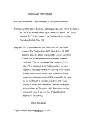
FIGURE 3.1 Total and Marginal Utility In the top panel, 

total utility (TU) increases by smaller and smaller amounts (the 

shaded areas) and so the marginal utility (MU) in the bottom 

panel declines. TU remains unchanged with the consumption of 

the fifth hamburger, and so MU is zero. After the fifth hamburger 

per day, TU declines and MU is negative. 

CHAPTER 3 Consumer Preferences and Choice 59 

22 

20 

16 

10 

Total utility of X TUX 

0 

12 

10 

8 

6 

4 

2 

0 

-2 

Marginal utility of X MUX 

1 2 3 4 5 6 Q X 

Quantity of X 

Plotting the values given in Table 3.1, we obtain Figure 3.1, with the top panel 

showing total utility and the bottom panel showing marginal utility. The total and marginal 

utility curves are obtained by joining the midpoints of the bars measuring TU and MU at 

each level of consumption. Note that the TU rises by smaller and smaller amounts (the 

shaded areas) and so the MU declines. The consumer reaches saturation after consuming 

TU X 

5 6 

1 2 3 4 

Q X 

Quantity of X MUX



Law of diminishing 

marginal utility Each 

additional unit of a good 

eventually gives less and 

less extra utility. 

✓ Concept Check 

What is the relationship 

between diminishing 

marginal utility and the 

law of demand? 

Cardinal utility An 

actual measure of 

utility, in util. 

Ordinal utility The 

rankings of the utility 

received from 

consuming various 

amounts of a good. 

the fourth hamburger. Thus, TU remains unchanged with the consumption of the fifth 

hamburger and MU is zero. After the fifth hamburger, TU declines and so MU is negative. 

The negative slope or downward-to-the-right inclination of the MU curve reflects the law 

of diminishing marginal utility. 

Utility schedules reflect tastes of a particular individual; that is, they are unique to 

the individual and reflect his or her own particular subjective preferences and perceptions. 

Different individuals may have different tastes and different utility schedules. 

Utility schedules remain unchanged so long as the individual’s tastes remain the same. 

Cardinal or Ordinal Utility? 

The concept of utility discussed in the previous section was introduced at about the same 

time, in the early 1870s, by William Stanley Jevons of Great Britain, Carl Menger of 

Austria, and Léon Walras of France. They believed that the utility an individual receives 

from consuming each quantity of a good or basket of goods could be measured cardinally 

just like weight, height, or temperature. 2 

Cardinal utility means that an individual can attach specific values or numbers of 

utils from consuming each quantity of a good or basket of goods. In Table 3.1 we saw 

that the individual received 10 utils from consuming one hamburger. He received 16 

utils, or 6 additional utils, from consuming two hamburgers. The consumption of the 

third hamburger gave this individual 4 extra utils, or two-thirds as many extra utils, as 

the second hamburger. Thus, Table 3.1 and Figure 3.1 reflect cardinal utility. They actually 

provide an index of satisfaction for the individual. 

In contrast, ordinal utility only ranks the utility received from consuming 

various amounts of a good or baskets of goods. Ordinal utility specifies that consuming 

two hamburgers gives the individual more utility than when consuming 

one hamburger, but it does not specify exactly how much additional utility the second 

hamburger provides. Similarly, ordinal utility would say only that three hamburgers 

give this individual more utility than two hamburgers, but not how many 

more utils. 3 

Ordinal utility is a much weaker notion than cardinal utility because it only 

requires that the consumer be able to rank baskets of goods in the order of his or her 

preference. That is, when presented with a choice between any two baskets of goods, 

ordinal utility requires only that the individual indicate if he or she prefers the first basket, 

the second basket, or is indifferent between the two. It does not require that the 

individual specify how many more utils he or she receives from the preferred basket. In 

short, ordinal utility only ranks various consumption bundles, whereas cardinal utility 

provides an actual index or measure of satisfaction. 

2 A market basket of goods can be defined as containing specific quantities of various goods and services. For 

example, one basket may contain one hamburger, one soft drink, and a ticket to a ball game, while another 

basket may contain two soft drinks and two movie tickets. 

3 To be sure, numerical values could be attached to the utility received by the individual from consuming 

various hamburgers, even with ordinal utility. However, with ordinal utility, higher utility values only 

indicate higher rankings of utility, and no importance can be attached to actual numerical differences in 

utility. For example, 20 utils can only be interpreted as giving more utility than 10 utils, but not twice as 

much. Thus, to indicate rising utility rankings, numbers such as 5, 10, 20; 8, 15, 17; or I (lowest), II, and III 

are equivalent.



What is the distinction 

between cardinal and 

ordinal utility? 

EXAMPLE 3–1 

Does Money Buy Happiness? 


How much money do 

you need to be happy? 


The distinction between cardinal and ordinal utility is important because a theory 

of consumer behavior can be developed on the weaker assumption of ordinal utility 

without the need for a cardinal measure. And a theory that reaches the same conclusion 

as another on weaker assumptions is a superior theory. 4 Utility theory provides a convenient 

introduction to the analysis of consumer tastes and to the more rigorous indifference 

curve approach. It is also useful for the analysis of consumer choices in the face 

of uncertainty, which is presented in Chapter 6. Example 3–1 examines the relationship 

between money income and happiness. 

Does money buy happiness? Philosophers have long pondered this question. 

Economists have now gotten involved in trying to answer this age-old question. They 

calculated the “mean happiness rating” (based on a score of “very happy” = 4, 

“pretty happy” = 2, and “not too happy” = 0) for individuals at different levels of personal 

income at a given point in time and for different nations over time. What they 

found was that up to an income per capita of about $20,000, higher incomes in the 

United States were positively correlated with happiness responses, but that after that, 

higher incomes had little, if any, effect on observed happiness. Furthermore, average 

individual happiness in the United States remained remarkably flat since the 1950s in 

the face of a considerable increase in average income. Similar results were found for 

other advanced nations, such as the United Kingdom, France, Germany, and Japan. 

These results seem to go counter to the basic economic assumption that higher personal 

income leads to higher utility. 

Two explanations are given for these remarkable and puzzling results: (1) that 

happiness is based on relative rather than absolute income and (2) that happiness 

quickly adapts to changes in the level of income. Specifically, higher incomes make 

individuals happier for a while, but their effect fades very quickly as individuals adjust 

to the higher income and soon take it for granted. For example, a generation ago, central 

heating was regarded as a luxury, while today it is viewed as essential. 

Furthermore, as individuals become richer, they become happier, but when society as 

a whole grows richer, nobody seems happier. In other words, people are often more 

concerned about their income relative to others’ than about their absolute income. 

Pleasure at your own pay rise can vanish when you learn that a colleague has been 

given a similar pay increase. 

The implication of all of this is that people’s effort to work more in order to earn 

and spend more in advanced (rich) societies does not make people any happier because 

others do the same. (In poor countries, higher incomes do make people happier). 

Lower taxes in the United States encourage people to work more and the nation to 

grow faster than in Europe, but this does not necessarily make Americans happier than 

4 This is like producing a given output with fewer or cheaper inputs, or achieving the same medical result 

(such as control of high blood pressure) with less or weaker medication.



3.2 

Good A commodity of 

which more is preferred 

to less. 

Bad An item of which 

less is preferred to more. 

Indifference curve 

The curve showing the 

various combinations of 

two commodities that 

give the consumer 

equal satisfaction. 

Europeans. The consensus among happiness researchers is that after earning enough to 

satisfy basic wants (a per capita income of about $20,000), family, friends, and community 

tend to be the most important things in life. 

Sources: R. A. Easterlin, “Income and Happiness,” Economic Journal, July 2000; B. S. Frey and A. 

Stutzer, “What Can Economists Learn from Happiness Research?,” Journal of Economic Literature, June 

2002; R. Layard, Happiness: Lessons from a New Science (London: Penguin, 2005); R. Di Tella and 

R. MacCulloch, “Some Uses of Happiness Data, Journal of Economic Perspectives, Winter 2006, 

pp. 25–46; and A. E. Clark, P. Frijters, and M. A. Shields, “Relative Income, Happiness, and Utility: 

An Explanation for the Easterlin Paradox and Other Puzzles,” Journal of Economic Literature, March 

2008, pp. 95–144. 

CONSUMER’S TASTES: INDIFFERENCE CURVES 

In this section, we define indifference curves and examine their characteristics. 

Indifference curves were first introduced by the English economist F. Y. Edgeworth in the 

1880s. The concept was refined and used extensively by the Italian economist Vilfredo 

Pareto in the early 1900s. Indifference curves were popularized and greatly extended in 

application in the 1930s by two other English economists: R. G. D. Allen and John R. 

Hicks. Indifference curves are a crucial tool of analysis because they are used to represent 

an ordinal measure of the tastes and preferences of the consumer and to show how the 

consumer maximizes utility in spending income. 

Indifference Curves—What Do They Show? 5 

Consumers’ tastes can be examined with ordinal utility. An ordinal measure of utility is 

based on three assumptions. First, we assume that when faced with any two baskets of 

goods, the consumer can determine whether he or she prefers basket A to basket B, B to A, 

or whether he or she is indifferent between the two. Second, we assume that the tastes of 

the consumer are consistent or transitive. That is, if the consumer states that he or she 

prefers basket A to basket B and also that he or she prefers basket B to basket C, then that 

consumer will prefer A to C. Third, we assume that more of a commodity is preferred to 

less; that is, we assume that the commodity is a good rather than a bad, and the consumer 

is never satiated with the commodity. 6 The three assumptions can be used to represent an 

individual’s tastes with indifference curves. In order to conduct the analysis by plane 

geometry, we will assume throughout that there are only two goods, X and Y. 

An indifference curve shows the various combinations of two goods that give the 

consumer equal utility or satisfaction. A higher indifference curve refers to a higher level 

of satisfaction, and a lower indifference curve refers to less satisfaction. However, we 

have no indication as to how much additional satisfaction or utility a higher indifference 

curve indicates. That is, different indifference curves simply provide an ordering or ranking 

of the individual’s preference. 

5 For a mathematical presentation of indifference curves and their characteristics using rudimentary calculus, 

see Section A.1 of the Mathematical Appendix at the end of the book. 

6 Examples of bads are pollution, garbage, and disease, of which less is preferred to more.



Are the indifference 

curves of various 

individuals the same? 


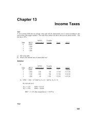
For example, Table 3.2 gives an indifference schedule showing the various combinations 

of hamburgers (good X) and soft drinks (good Y) that give the consumer equal satisfaction. 

This information is plotted as indifference curve U1 in the left panel of Figure 3.2. 

The right panel repeats indifference curve U1 along with a higher indifference curve (U2) 

and a lower one (U0). 

Indifference curve U1 shows that one hamburger and ten soft drinks per unit of time 

(combination A) give the consumer the same level of satisfaction as two hamburgers and six 

soft drinks (combination B), four hamburgers and three soft drinks (combination C ), or 

seven hamburgers and one soft drink (combination F). On the other hand, combination R 

(four hamburgers and seven soft drinks) has both more hamburgers and more soft drinks 

than combination B (see the right panel of Figure 3.2), and so it refers to a higher level of 

satisfaction. Thus, combination R and all the other combinations that give the same level of 

satisfaction as combination R define higher indifference curve U2. Finally, all combinations 

Soft drinks 

per unit 

of time 

TABLE 3.2 

(Y ) 

10 

6 

3 

1 

A 

Indifference Schedule 

Hamburgers (X) Soft Drinks (Y) Combinations 

1 10 A 

2 6 B 

4 3 C 

7 1 F 

B 

C 

U 1 

0 1 2 4 7 

Hamburgers (X ) per unit of time 

F 

Quantity of Y 

Q Y 

11 

10 

8 

7 

6 

5 

4 

3 

2 

1 

0 

T 

1 

A 

B 

2 3 

4 

R 

C 

U 0 

6 

7 

Quantity of X 

F U1 

FIGURE 3.2 Indifference Curves The individual is indifferent among combinations A, B, C, and F 

since they all lie on indifference curve U1. U1 refers to a higher level of satisfaction than U0, but to a 

lower level than U2. 

9 

U 2 

Q X



Indifference map 

The entire set of 

indifference curves 

reflecting the 

consumer’s tastes 

and preferences. 


Why are indifference 

curves negatively 

sloped? 

on U0 give the same satisfaction as combination T, and combination T refers to both fewer 

hamburgers and fewer soft drinks than (and therefore is inferior to) combination B on U1. 

Although in Figure 3.2 we have drawn only three indifference curves, there is an 

indifference curve going through each point in the XY plane (i.e., referring to each possible 

combination of good X and good Y). That is, between any two indifference curves, an 

additional curve can always be drawn. The entire set of indifference curves is called an 

indifference map and reflects the entire set of tastes and preferences of the consumer. 

Characteristics of Indifference Curves 

Indifference curves are usually negatively sloped, cannot intersect, and are convex to the 

origin (see Figure 3.2). Indifference curves are negatively sloped because if one basket of 

goods X and Y contains more of X, it will have to contain less of Y than another basket in 

order for the two baskets to give the same level of satisfaction and be on the same indifference 

curve. For example, since basket B on indifference curve U1 in Figure 3.2 contains 

more hamburgers (good X) than basket A, basket B must contain fewer soft drinks (good Y ) 

for the consumer to be on indifference curve U1. 

A positively sloped curve would indicate that one basket containing more of both 

commodities gives the same utility or satisfaction to the consumer as another basket containing 

less of both commodities (and no other commodity). Because we are dealing with 

goods rather than bads, such a curve could not possibly be an indifference curve. For 

example, in the left panel of Figure 3.3, combination B ′ contains more of X and more of Y 

than combination A ′ , and so the positively sloped curve on which B ′ and A ′ lie cannot be an 

indifference curve. That is, B ′ must be on a higher indifference curve than A ′ if X and Y are 

both goods. 7 

Quantity of Y 

Q Y 

0 

A9 

B9 

Quantity of X 

Q X 

Quantity of Y 

Q Y 

7 Only if either X or Y were a bad would the indifference curve be positively sloped as in the left panel of 

Figure 3.3. 

0 

2 

1 

A* 

Quantity of X 

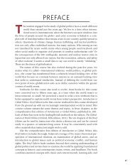
FIGURE 3.3 Indifference Curves Cannot Be Positively Sloped or Intersect 

In the left panel, the positively sloped curve cannot be an indifference curve because it 

shows that combination B ′′ , which contains more of X and Y than combination A ′ , gives 

equal satisfaction to the consumer as A ′ . In the right panel, since C* is on curves 1 and 2, 

it should give the same satisfaction as A* and B*, but this is impossible because B* has 

more of X and Y than A*. Thus, indifference curves cannot intersect. 

C* 

B* 

1 

2 

Q X


Marginal rate of 

substitution (MRS) 

The amount of a good 

that a consumer is 

willing to give up for an 

additional unit of 

another good while 

remaining on the same 

indifference curve. 


Indifference curves also cannot intersect. Intersecting curves are inconsistent with 

the definition of indifference curves. For example, if curve 1 and curve 2 in the right 

panel of Figure 3.3 were indifference curves, they would indicate that basket A* 

is equivalent to basket C* since both A* and C* are on curve 1, and also that basket 

B* is equivalent to basket C* since both B* and C* are on curve 2. By transitivity, B* 

should then be equivalent to A*. However, this is impossible because basket B* contains 

more of both good X and good Y than basket A*. Thus, indifference curves cannot 

intersect. 

Indifference curves are usually convex to the origin; that is, they lie above any tangent 

to the curve. Convexity results from or is a reflection of a decreasing marginal rate 

of substitution, which is discussed next. 

The Marginal Rate of Substitution 

The marginal rate of substitution (MRS) refers to the amount of one good that an individual 

is willing to give up for an additional unit of another good while maintaining the 

same level of satisfaction or remaining on the same indifference curve. For example, the 

marginal rate of substitution of good X for good Y (MRSXY) refers to the amount of Y that 

the individual is willing to exchange per unit of X and maintain the same level of satisfaction. 

Note that MRSXY measures the downward vertical distance (the amount of Y that the 

individual is willing to give up) per unit of horizontal distance (i.e., per additional unit of X 

required) to remain on the same indifference curve. That is, MRSXY =−∆Y/∆X. Because 

of the reduction in Y, MRSXY is negative. However, we multiply by −1 and express MRSXY 

as a positive value. 

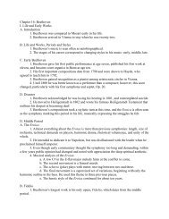
For example, starting at point A on U1 in Figure 3.4, the individual is willing to give 

up four units of Y for one additional unit of X and reach point B on U1. Thus, MRSXY = 

−(−4/1) = 4. This is the absolute (or positive value of the) slope of the chord from point 

A to point B on U1. Between point B and point C on U1, MRSXY = 3/2 = 1.5 (the absolute 

slope of chord BC ). Between points C and F, MRSXY = 2/3 = 0.67. At a particular point 

on the indifference curve, MRSXY is given by the absolute slope of the tangent to the indifference 

curve at that point. Different individuals usually have different indifference 

curves and different MRSXY (at points where their indifference curves have different 

slopes). 

We can relate indifference curves to the preceding utility analysis by pointing out that 

all combinations of goods X and Y on a given indifference curve refer to the same level of 

total utility for the individual. Thus, for a movement down a given indifference curve, the 

gain in utility in consuming more of good X must be equal to the loss in utility in consuming 

less of good Y. Specifically, the increase in consumption of good X (X) times the 

marginal utility that the individual receives from consuming each additional unit of X 

(MUX) must be equal to the reduction in Y (−Y) times the marginal utility of Y (MUY). 

That is, 

so that 

(X)(MUX) =−(Y)(MUY) [3.1] 

MUX/MUY =−Y/X = MRSXY 

[3.2] 

Thus, MRSXY is equal to the absolute slope of the indifference curve and to the ratio of the 

marginal utilities.



FIGURE 3.4 Marginal Rate of Substitution (MRS) Starting at 

point A, the individual is willing to give up 4 units of Y for one 

additional unit of X and reach point B on U1. Thus, MRSXY = 4 (the 

absolute slope of chord AB). Between points B and C, MRSXY = 

3/2. Between C and F, MRSXY = 2/3. MRSXY declines as the 

individual moves down the indifference curve. 

Quantity of Y 

Q Y 

Note that MRSXY (i.e., the absolute slope of the indifference curve) declines as we 

move down the indifference curve. This follows from, or is a reflection of, the convexity 

of the indifference curve. That is, as the individual moves down an indifference curve and 

is left with less and less Y (say, soft drinks) and more and more X (say, hamburgers), each 

remaining unit of Y becomes more valuable to the individual and each additional unit of 

X becomes less valuable. Thus, the individual is willing to give up less and less of Y to 

obtain each additional unit of X. It is this property that makes MRSXY diminish and indifference 

curves convex to the origin. We will see in Section 3.5 the crucial role that convexity 

plays in consumer utility maximization. 8 

Some Special Types of Indifference Curves 

10 

6 

3 

1 

0 

4 6 

Quantity of X 

7 Q X 

Although indifference curves are usually negatively sloped and convex to the origin, 

they may sometimes assume other shapes, as shown in Figure 3.5. Horizontal indifference 

curves, as in the top left panel of Figure 3.5, would indicate that commodity X is 

a neuter; that is, the consumer is indifferent between having more or less of the 

commodity. Vertical indifference curves, as in the top right panel of Figure 3.5, would 

indicate instead that commodity Y is a neuter. 

The bottom left panel of figure 3.5 shows indifference curves that are negatively 

sloped straight lines. Here, MRSXY or the absolute slope of the indifference curves is constant. 

This means that an individual is always willing to give up the same amount of good 

Y (say, two cups of tea) for each additional unit of good X (one cup of coffee). Therefore, 

good X and two units of good Y are perfect substitutes for this individual. 

8 A movement along an indifference curve in the upward direction measures MRSYX, which also diminishes. 

–4Y 

1 

A 

1X 

–3Y 

2 

B 

2X 

–2Y 

C 

3X 

F 

U 1


6 

U 2 

U 1 

U 0 

0 2 4 6 Q X 


Q Y Q Y U0 U1 U2 4 

2 

Q Y 

8 

6 

4 

2 

U 0 

U 1 

U 2 

0 2 4 6 8 Q X 

6 

4 

2 

Q Y 

0 2 4 6 Q X 

10 

8 

6 

3 

A 

B 

U 0 

C 

U 1 

U 2 

F 

0 2 4 6 Q X 

FIGURE 3.5 Some Unusual Indifference Curves Horizontal indifference curves, 

as in the top left panel, indicate that X is a neuter; that is, the consumer is indifferent 

between having more or less of it. Vertical indifference curves, as in the top right 

panel, would indicate instead that commodity Y is a neuter. Indifference curves that 

are negatively sloped straight lines, as in the bottom left panel, indicate that MRSXY is 

constant, and so X and Y are perfect substitutes for the individual. The bottom right 

panel shows indifference curves that are concave to the origin (i.e., MRSXY increases). 

Finally, the bottom right panel shows indifference curves that are concave rather than 

convex to the origin. This means that the individual is willing to give up more and more 

units of good Y for each additional unit of X (i.e., MRSXY increases). For example, 

between points A and B on U1, MRSXY = 2/2 = 1; between B and C, MRSXY = 3/1 = 3; 

and between C and F, MRSXY = 3/0.5 = 6. In Section 3.5, we will see that in this unusual 

case, the individual would end up consuming only good X or only good Y. 

Even though indifference curves can assume any of the shapes shown in Figure 3.5, 

they are usually negatively sloped, nonintersecting, and convex to the origin. These characteristics 

have been confirmed experimentally. 9 Because it is difficult to derive indifference 

curves experimentally, however, firms try to determine consumers’ preferences by 

marketing studies, as explained in Example 3–2. 

9 See, for example, K. R. MacCrimmon and M. Toda, “The Experimental Determination of Indifference 

Curves,” Review of Economic Studies, October 1969.



EXAMPLE 3–2 

How Ford Decided on the Characteristics of Its Taurus 

Firms can learn about consumers’ preferences by conducting or commissioning marketing 

studies to identify the most important characteristics of a product, say, styling and 

performance for automobiles, and to determine how much more consumers would be 

willing to pay to have more of each attribute, or how they would trade off more of one 

attribute for less of another. This approach to consumer demand theory, which focuses 

on the characteristics or attributes of goods and on their worth or hedonic prices rather 

than on the goods themselves, was pioneered by Kelvin Lancaster (see “At the Frontier” 

in Chapter 4). This is in fact how the Ford Motor Company decided on the characteristics 

of its 1986 Taurus. 

Specifically, Ford determined by marketing research that the two most important 

characteristics of an automobile for the majority of consumers were styling (i.e., 

design and interior features) and performance (i.e., acceleration and handling) and 

then produced its Taurus in 1986 that incorporated those characteristics. The rest is 

history (the Taurus regained in 1992 its status of the best-selling car in America—a 

position that it had lost to the Honda Accord in 1989). Ford also used this approach to 

decide on the characteristics of the all-new 1996 Taurus, the first major overhaul since 

its 1986 launch, at a cost of $2.8 billion, as well as in deciding the characteristics of its 

world cars, Focus, launched in 1998, the Mondeo introduced in 2000, and the new 

Fiesta in Europe in 2008 and in the United States in 2010. Other automakers, such as 

General Motors, followed similar procedures in determining the characteristics of 

their automobiles. Since then U.S. automakers have shifted somewhat toward producing 

“sports wagons,” which are a cross between sedans and sport-utility vehicles 

(SUVs) to reflect recent changes in consumer tastes, and toward more fuel-efficient 

and “green” automobiles as a result of the sharp increase in gasoline prices and heightened 

environmental concerns. 

Market studies can also be used to determine how consumers’ tastes have changed 

over time. In terms of indifference curves, a reduction in the consumer’s taste for commodity 

X (hamburgers) in relation to commodity Y (soft drinks) would be reflected in 

a flattening of the indifference curve of Figure 3.4, indicating that the consumer would 

now be willing to give up less of Y for each additional unit of X. The different tastes of 

different consumers are also reflected in the shapes of their indifference curves. The 

consumer who prefers soft drinks to hamburgers will have a flatter indifferences curve 

than a consumer who does not. 

Sources: “Ford Puts Its Future on the Line,” New York Times Magazine, December 4, 1985, pp. 94–110; 

V. Bajic, “Automobiles and Implicit Markets: An Estimate of a Structural Demand Model for Automobile 

Characteristics,” Applied Economics, April 1993, pp. 541–551; “Ford Hopes Its New Focus Will Be a 

Global Best Seller,” Wall Street Journal, October 8, 1998, p. B10; S. Berry, J. Levinsohn, and A. Pakes, 

“Differentiated Products Demand Systems from a Combination of Macro and Micro Data: The New Car 

Market,” National Bureau of Economic Research, Working Paper 6481, March 1998; and “Ford’s Taurus 

Loses Favor to New-Age Sport Wagon,” New York Times, February 7, 2002, p. B1; “Once Frumpy, Green 

Cars Start Showing Some Flash,” New York Times, July 15, 2007, p. 13; “Ford Eyes More Cuts, as 

Recovery Advances,” Wall Street Journal, April 23, 2008, p. A1; and “One World, One Car, One Name,” 

Business Week, March 24, 2008, p. 63.


3.3 

EXAMPLE 3–3 

INTERNATIONAL CONVERGENCE OF TASTES 


A rapid convergence of tastes is taking place in the world today. Tastes in the United 

States affect tastes around the world and tastes abroad strongly influence tastes in the 

United States. Coca-Cola and jeans are only two of the most obvious U.S. products that 

have become household items around the world. One can see Adidas sneakers and 

Walkman personal stereos on joggers from Central Park in New York City to Tivoli 

Gardens in Copenhagen. You can eat Big Macs in Piazza di Spagna in Rome or Pushkin 

Square in Moscow. We find Japanese cars and VCRs in New York and in New Delhi, 

French perfumes in Paris and in Cairo, and Perrier in practically every major (and not so 

major) city around the world. Texas Instruments and Canon calculators, Dell and Hitachi 

portable PCs, and Xerox and Minolta copiers are found in offices and homes more or less 

everywhere. With more rapid communications and more frequent travel, the worldwide 

convergence of tastes has even accelerated. This has greatly expanded our range of consumer 

choices and forced producers to think in terms of global production and marketing 

to remain competitive in today’s rapidly shrinking world. 

In his 1983 article “The Globalization of Markets” in the Harvard Business Review, 

Theodore Levitt asserted that consumers from New York to Frankfurt to Tokyo want similar 

products and that success for producers in the future would require more and more 

standardized products and pricing around the world. In fact, in country after country, we 

are seeing the emergence of a middle-class consumer lifestyle based on a taste for comfort, 

convenience, and speed. In the food business, this means packaged, fast-to-prepare, 

and ready-to-eat products. Market researchers have discovered that similarities in living 

styles among middle-class people all over the world are much greater than we once 

thought and are growing with rising incomes and education levels. Of course, some differences 

in tastes will always remain among people of different nations, but with the 

tremendous improvement in telecommunications, transportation, and travel, the crossfertilization 

of cultures and convergence of tastes can only be expected to accelerate. This 

trend has important implications for consumers, producers, and sellers of an increasing 

number and types of products and services. 

Gillette Introduces the Sensor and Mach3 Razors—Two Truly 

Global Products 

As tastes become global, firms are responding more and more with truly global 

products. These are introduced more or less simultaneously in most countries of the 

world with little or no local variation. This is leading to what has been aptly called 

the “global supermarket.” For example, in 1990, Gillette introduced its new Sensor 

Razor at the same time in most nations of the world and advertised it with virtually 

the same TV spots (ad campaign) in 19 countries in Europe and North America. 

In 1994, Gillette introduced an upgrade of the Sensor Razor called SensorExcell




Why are tastes 

converging 

internationally? 

3.4 

with a high-tech edge. By 1998, Gillette had sold over 400 million of Sensor and 

SensorExcell razors and more than 8 billion twin-blade cartridges, and it had captured 

an incredible 71% of the global blade market. Then in April 1998, Gillette unveiled 

the Mach3, the company’s most important new product since the Sensor. It has three 

blades with a new revolutionary edge produced with chipmaking technology that 

took five years to develop. Gillette developed its new razor in stealth secrecy at the 

astounding cost of over $750 million, and spent another $300 million to advertise it. 

Since it went on sale in July 1998, the Mach3 has proven to be an even greater success 

than the Sensor Razor. Gillette introduced the Mach3 Turbo Razor worldwide 

in April 2002, in June 2004 its M3Power Razor, as an evolution of its Mach 3, and 

its five-blade Fusion in early 2006. With the merger of Gillette and Procter & 

Gamble, the global reach of the M3Power and Fusion are likely to be even greater 

than for its predecessors. 

The trend toward the global supermarket is rapidly spreading in Europe as borders 

fade and as Europe’s single currency (the euro) brings prices closer across the 

continent. A growing number of companies are creating “Euro-brands”—a single 

product for most countries of Europe—and advertising them with “Euro-ads,” which 

are identical or nearly identical across countries, except for language. Many national 

differences in taste will, of course, remain; for example, Nestlé markets more than 

200 blends of Nescafé to cater to differences in tastes in different markets. But the 

converging trend in tastes around the world is unmistakable and is likely to lead to 

more and more global products. This is true not only in foods and inexpensive consumer 

products but also in automobiles, tires, portable computers, phones, and many 

other durable products. 

Sources: “Building the Global Supermarket,” New York Times, November 18, 1988, p. D1; “Gillette’s 

World View: One Blade Fits All,” Wall Street Journal, January 3, 1994, p. C3; “Gillette Finally Reveals 

Its Vision of the Future, and it Has 3 Blades,” Wall Street Journal, April 4, 1998, p. A1; “Gillette, 

Defying Economy, Introduces a $9 Razor Set,” New York Times, October 31, 2001, p. C4; “Selling in 

Europe: Borders Fade,” New York Times, May 31, 1990, p. D1; “Converging Prices Mean Trouble for 

European Retailers,” Financial Times, June 18, 1999, p. 27; “Can Nestlé Be the Very Best?,” Fortune, 

November 13, 2001, pp. 353–360; “For Cutting-Edge Dads,” US News & World Report, June 14, 2004, 

pp. 80–81; “P&G’s $57 Billion Bargain,” BusinessWeek, July 25, 2005, p. 26; and “How Many Blades 

Is Enough?” Fortune, October 31, 2005, p. 40; and “Gillette New Edge,” Business Week, February 6, 

2006, p. 44. 

THE CONSUMER’S INCOME AND PRICE CONSTRAINTS: 

THE BUDGET LINE 

In this section, we introduce the constraints or limitations faced by a consumer in satisfying 

his or her wants. In order to conduct the analysis by plane geometry, we assume 

that the consumer spends all of his or her income on only two goods, X and Y. We will 

see that the constraints of the consumer can then be represented by a line called the budget 

line. The position of the budget line and changes in it can best be understood by 

looking at its endpoints.


Budget constraint 

The limitation on the 

amount of goods that a 

consumer can purchase 

imposed by his or her 

limited income and the 

prices of the goods. 

Budget line A line 

showing the various 

combinations of two 

goods that a consumer 

can purchase by 

spending all income. 

Definition of the Budget Line 


In Section 3.2, we saw that we can represent a consumer’s tastes with an indifference 

map. We now introduce the constraints or limitations that a consumer faces in attempting 

to satisfy his or her wants. The amount of goods that a consumer can purchase over a 

given period of time is limited by the consumer’s income and by the prices of the goods 

that he or she must pay. In what follows we assume (realistically) that the consumer cannot 

affect the price of the goods he or she purchases. In economics jargon, we say that the 

consumer faces a budget constraint due to his or her limited income and the given prices 

of goods. 

By assuming that a consumer spends all of his or her income on good X (hamburgers) 

and on good Y (soft drinks), we can express the budget constraint as 

PXQX + PYQY = I [3.3] 

where PX is the price of good X, QX is the quantity of good X, PY is the price of good Y, 

QY is the quantity of good Y, and I is the consumer’s money income. Equation [3.3] postulates 

that the price of X times the quantity of X plus the price of Y times the quantity of 

Y equals the consumer’s money income. That is, the amount of money spent on X plus 

the amount spent on Y equals the consumer’s income. 10 

Suppose that PX = $2, PY = $1, and I = $10 per unit of time. This could, for example, 

be the situation of a student who has $10 per day to spend on snacks of hamburgers 

(good X) priced at $2 each and on soft drinks (good Y) priced at $1 each. By spending all 

income on Y, the consumer could purchase 10Y and 0X. This defines endpoint J on the 

vertical axis of Figure 3.6. Alternatively, by spending all income on X, the consumer 

could purchase 5X and 0Y. This defines endpoint K on the horizontal axis. By joining endpoints 

J and K with a straight line we get the consumer’s budget line. This line shows the 

various combinations of X and Y that the consumer can purchase by spending all income 

at the given prices of the two goods. For example, starting at endpoint J, the consumer 

could give up two units of Y and use the $2 not spent on Y to purchase the first unit of X 

and reach point L. By giving up another 2Y, he or she could purchase the second unit of 

X. The slope of −2 of budget line JK shows that for each 2Y the consumer gives up, he or 

she can purchase 1X more. 

By rearranging equation [3.3], we can express the consumer’s budget constraint in a 

different and more useful form, as follows. By subtracting the term PXQX from both sides 

of equation [3.3] we get 

PYQY = I − PXQX 

10 Equation [3.3] could be generalized to deal with any number of goods. However, as pointed out, we deal 

with only two goods for purposes of diagrammatic analysis. 

[3.3A] 

By then dividing both sides of equation [3.3A] by PY, we isolate QY on the left-hand side 

and define equation [3.4]: 

QY = I/PY − (PX /PY)QX 

[3.4]



FIGURE 3.6 The Budget Line With an income of I = 

$10, and PY = $1 and PX = $2, we get budget line JK. This 

shows that the consumer can purchase10Y and 0X (endpoint 

J), 8Y and1X (point L), 6Y and 2X (point B),or...0Y and 5X 

(endpoint K). I/PY = $10/$1 = 10 is the vertical or Y-intercept 

of the budget line and −PX/PY =−$2/$1 =−2 is the slope. 

The first term on the right-hand side of equation [3.4] is the vertical or Y-intercept of the 

budget line and −PX /PY is the slope of the budget line. For example, continuing to use PX 

= $2, PY = $1, and I = $10, we get I /PY = 10 for the Y-intercept (endpoint J in Figure 

3.6) and −PX /PY = −2 for the slope of the budget line. The slope of the budget line refers 

to the rate at which the two goods can be exchanged for one another in the market (i.e., 2Y 

for 1X). 

The consumer can purchase any combination of X and Y on the budget line or in the 

shaded area below the budget line (called budget space). For example, at point B the individual 

would spend $4 to purchase 2X and the remaining $6 to purchase 6Y. At point M, 

he or she would spend $8 to purchase 4X and the remaining $2 to purchase 2Y. On the 

other hand, at a point such as H in the shaded area below the budget line (i.e., in the budget 

space), the individual would spend $4 to purchase 2X and $3 to purchase 3Y and be 

left with $3 of unspent income. In what follows, we assume that the consumer does spend 

all of his or her income and is on the budget line. Because of the income and price constraints, 

the consumer cannot reach combinations of X and Y above the budget line. For 

example, the individual cannot purchase combination G (4X, 6Y) because it requires an 

expenditure of $14 ($8 to purchase 4X plus $6 to purchase 6Y). 

Changes in Income and Prices and the Budget Line 

A particular budget line refers to a specific level of the consumer’s income and specific 

prices of the two goods. If the consumer’s income and/or the price of good X or good Y 

change, the budget line will also change. When only the consumer’s income changes, the 

budget line will shift up if income (I ) rises and down if I falls, but the slope of the budget 

line remains unchanged. For example, the left panel of Figure 3.7 shows budget line JK 

(the same as in Figure 3.6 with I = $10), higher budget line J ′ K ′ with I = $15, and still 

higher budget line J ′′ K ′′ with I = $20 per day. PX and PY do not change, so the three budget 

lines are parallel and their slopes are equal. If the consumer’s income falls, the budget 

line shifts down but remains parallel. 

Quantity of Y 

Q Y 

10 

8 

6 

3 

2 

J 

L 

B G 

H 

M 

K 

0 1 2 4 5 Q X 

Quantity of X



What happens to the 

budget line if the price 

of Y falls more than the 

price of X? 

Q Y 

20 

15 

10 

0 

J" 

J 9 

J 

K 

K9 

5 7.5 10 

K" 

Q X 

Q Y 

10 

J 


If only the price of good X changes, the vertical or Y-intercept remains unchanged, 

and the budget line rotates upward or counterclockwise if PX falls and downward or 

clockwise if PX rises. For example, the right panel of Figure 3.7 shows budget line JK (the 

same as in Figure 3.6 at PX = $2), budget line JK ′′ with PX = $1, and budget line JN ′ with 

PX = $0.50. The vertical intercept (endpoint J) remains the same because I and PY do not 

change. The slope of budget line JK ′′ is −PX /PY = −$1=$1 =−1. The slope of budget 

line JN ′ is −1/2. With an increase in PX, the budget line rotates clockwise and becomes 

steeper. 

On the other hand, if only the price of Y changes, the horizontal or X-intercept will 

be the same, but the budget line will rotate upward if PY falls and downward if PY rises. 

For example, with I = $10, PX = $2, and PY = $0.50 (rather than PY = $1), the new vertical 

or Y-intercept is QY = 20 and the slope of the new budget line is −PX /PY = −4. 

With PY = $2, the new Y-intercept is QY = 5 and −PX=PY = −1 (you should be able to 

sketch these lines). Finally, with a proportionate reduction in PX and PY and constant I, 

there will be a parallel upward shift in the budget line; with a proportionate increase in 

PX and PY and constant I, there will be a parallel downward shift in the budget line. 

Example 3–4 shows that time, instead of the consumer’s income, can be a constraint. 

0 

K 

K" 

N9 

5 10 20 Q X 

FIGURE 3.7 Changes in the Budget Line The left panel shows budget line JK (the same as in Figure 3.6 

with I = $10), higher budget lineJ ′ K ′ with I = $15, and still higher budget line J ′′ K ′′ with I = $20 per day. PX and 

PY do not change, so the three budget lines are parallel and their slopes are equal. The right panel shows budget 

line JK with PX = $2, budget line JK ′′ with PX = $1, and budget line JN ′′ with PX = $0.50. The vertical or 

Y-intercept (endpoint J) remains the same because income and PY do not change. The slope of budget line JK ′′ 

is −PX /PY =−$1/$1 =−1, while the slope of budget line JN ′ is −1/2.



EXAMPLE 3–4 

Time as a Constraint 

3.5 

Rational consumer An 

individual who seeks to 

maximize utility or 

satisfaction in spending 

his or her income. 

In the preceding discussion of the budget line, we assumed only two constraints: the 

consumers’ income and the given prices of the two goods. In the real world, consumers 

are also likely to face a time constraint. That is, since the consumption of 

goods requires time, which is also limited, time often represents another constraint 

faced by consumers. This explains the increasing popularity of precooked or readyto-eat 

foods, restaurant meals delivered at home, and the use of many other time-saving 

goods and services. But the cost of saving time can be very expensive—thus 

proving the truth of the old saying that “time is money.” 

For example, the food industry is introducing more and more foods that are easy 

and quick to prepare, but these foods carry with them a much higher price. A meal 

that could be prepared from scratch for a few dollars might cost instead more than 

$10 in its ready-to-serve variety which requires only a few minutes to heat up. More 

and more people are also eating out and incurring much higher costs in order to save 

the time it takes to prepare home meals. McDonald’s, Burger King, Taco Bell, and 

other fast-food companies are not just selling food, but fast food, and for that customers 

are willing to pay more than for the same kind of food at traditional food outlets, 

which require more waiting time. Better still, many suburbanites are increasingly 

reaching for the phone, not the frying pan, at dinner time to arrange for the home 

delivery of restaurant meals, adding even more to the price or cost of a meal. 

Time is also a factor in considering transportation costs and access to the Internet. 

You could travel from New York to Washington, D.C., by train or, in less time but at a 

higher cost, by plane. Similarly, you can access the Internet with a regular but slow 

telephone line or much faster, but at a higher cost, by DSL or fiber optics. 

Sources: “Suburban Life in the Hectic 1990s: Dinner Delivered,” New York Times, November 20, 1992, 

p. B1; “How Much Will People Pay to Save a Few Minutes of Cooking? Plenty,” Wall Street Journal, 

July 25, 1985, p. B1; “Riding the Rails at What Price,” New York Times, June 18, 2001, p. 12; and 

“Shining Future for Fiber Optics,” New York Times, November 19, 1995, p. B10. 

CONSUMER’S CHOICE 

We will now bring together the tastes and preferences of the consumer (given by his or her 

indifference map) and the income and price constraints faced by the consumer (given by 

his or her budget line) to examine how the consumer determines which goods to purchase 

and in what quantities to maximize utility or satisfaction. As we will see in the next chapter, 

utility maximization is essential for the derivation of the consumer’s demand curve for 

a commodity (which is a major objective of this part of the text). 

Utility Maximization 

Given the tastes of the consumer (reflected in his or her indifference map), the rational 

consumer seeks to maximize the utility or satisfaction received in spending his or her 

income. A rational consumer maximizes utility by trying to attain the highest indifference


Constrained utility 

maximization The 

process by which the 

consumer reaches the 

highest level of 

satisfaction given his or 

her income and the 

prices of goods. 


Why is utility not 

maximized if the 

indifference curve 

crosses the budget 

line twice? 


curve possible, given his or her budget line. This occurs where an indifference curve is tangent 

to the budget line so that the slope of the indifference curve (the MRSXY) is equal to 

the slope of the budget line (PX/PY). Thus, the condition for constrained utility maximization, 

consumer optimization, or consumer equilibrium occurs where the consumer 

spends all income (i.e., he or she is on the budget line) and 

MRSXY = PX/PY 

[3.5] 

Figure 3.8 brings together on the same set of axes the consumer indifference curves 

of Figure 3.2 and the budget line of Figure 3.6 to determine the point of utility maximization. 

Figure 3.8 shows that the consumer maximizes utility at point B where indifference 

curve U1 is tangent to budget line JK. At point B, the consumer is on the budget line and 

MRSXY = PX/PY = 2. Indifference curve U1 is the highest that the consumer can reach with 

his or her budget line. Thus, to maximize utility the consumer should spend $4 to purchase 

2X and the remaining $6 to purchase 6Y. Any other combination of goods X and Y that the 

consumer could purchase (those on or below the budget line) provides less utility. For 

example, the consumer could spend all income to purchase combination L, but this would 

be on lower indifference curve U0. 

At point L the consumer is willing to give up more of Y than he or she has to in the 

market to obtain one additional unit of X. That is, MRSXY (the absolute slope of indifference 

curve U0 at point L) exceeds the value of PX/PY (the absolute slope of budget line 

JK). Thus, starting from point L, the consumer can increase his or her satisfaction by 

purchasing less of Y and more of X until he or she reaches point B on U1, where the slopes 

of U1 and the budget line are equal (i.e., MRSXY = PX/PY = 2). On the other hand, starting 

from point M, where MRSXY < PX/PY, the consumer can increase his or her satisfaction 

by purchasing less of X and more of Y until he or she reaches point B on U1, where 

MRSXY = PX/PY. One tangency point such as B is assured by the fact that there is an 

indifference curve going through each point in the XY commodity space. The consumer 

FIGURE 3.8 Constrained Utility Maximization The consumer 

maximizes utility at point B, where indifference curve U1 is tangent to 

budget line JK. At point B, MRSXY = PX/PY = 2. Indifference curve U1 is 

the highest that the consumer can reach with his or her budget line. 

Thus, the consumer should purchase 2X and 6Y. 

Quantity of Y 

Q Y 

10 

8 

6 

3 

J 

L 

B 

M 

U 

K 0 

U 1 

0 2 5 9 

Quantity of X 

U 2 

Q X



cannot reach indifference curve U2 with the present income and the given prices of 

goods X and Y. 11 

Utility maximization is more prevalent (as a general aim of individuals) than it may 

at first seem. It is observed not only in consumers as they attempt to maximize utility in 

spending income but also in many other individuals—including criminals. For example, 

a study found that the rate of robberies and burglaries was positively related to the gains 

and inversely related to the costs of (i.e., punishment for) criminal activity. 12 Utility maximization 

can also be used to analyze the effect of government warnings on consumption, 

as Example 3–5 shows. 

EXAMPLE 3–5 

Utility Maximization and Government Warnings on Junk Food 

Suppose that in Figure 3.9, good X refers to milk and good Y refers to soda, PX = $1, 

PY = $1, and the consumer spends his or her entire weekly allowance of $10 on milk 

and sodas. Suppose also that the consumer maximizes utility by spending $3 to purchase 

three containers of milk and $7 to purchase seven sodas (point B on indifference 

curve U1) before any government warning on the danger of dental cavities and obesity 

from sodas. After the warning, the consumer’s tastes may change away from sodas and 

toward milk. It may be argued that government warnings change the information available 

to consumers rather than tastes; that is, the warning affects consumers’ perception 

FIGURE 3.9 Effect of Government Warnings The 

consumer maximizes utility by purchasing 3 containers of milk 

and 7 sodas (point B on indifference curve U1) before the 

government warning on the consumption of sodas. After the 

warning, the consumer’s tastes change and are shown by dashed 

indifference curves U ′ 0 and U ′ 1. The consumer now maximizes 

utility by purchasing 6 containers of milk and only 4 sodas (point 

B ′ , where U ′ 1 is tangent to the budget line). 

Soda 

Q Y 

10 

7 

4 

0 

11 For a mathematical presentation of utility maximization using rudimentary calculus, see Section A.2 of 

the Mathematical Appendix. 

12 See I. Ehrlich, “Participation in Illegitimate Activities: A Theoretical and Empirical Investigation,” Journal 

of Political Economy, May/June 1973; W. T. Dickens, “Crime and Punishment Again: The Economic 

Approach with a Psychological Twist,” National Bureau of Economic Research, Working Paper No. 1884, 

April 1986; and A. Gaviria, “Increasing Returns and the Evolution of Violent Crimes: The Case of 

Colombia,” Journal of Development Economics, February 2000. 

3 

B 

B9 

U 1 

6 10 Q X 

Milk 

U 19 

U 09


Corner solution 

Constrained utility 

maximization with the 

consumer spending 

all of his or her income 

on only one or some 

goods. 


as to the ability of various goods to satisfy their wants—see M. Shodell, “Risky 

Business,” Science, October 1985. 

The effect of the government warning can be shown with dashed indifference 

curves U ′ 0 and U ′ 1. Note that U ′ 0 is steeper than U1 at than original optimization point 

B, indicating that after the warning the individual is willing to give up more sodas for 

an additional container of milk (i.e., MRSXY is higher for U ′ 0 than for U1 at point B). 

Now U ′ 0 can intersect U1 because of the change in tastes. Note also that U ′ 0 involves 

less utility than U1 at point B because the seven sodas (and the three containers of 

milk) provide less utility after the warning. After the warning, the consumer maximizes 

utility by consuming six containers of milk and only four sodas (point B ′ , 

where U ′ 1 is tangent to the budget line). 

The above analysis clearly shows how indifference curve analysis can be used to 

examine the effect of any government warning on consumption patterns, such as the 

1965 law requiring manufacturers to print on each pack of cigarettes sold in the United 

States the warning that cigarette smoking is dangerous to health. Indeed, the World 

Health Organization is now stepping up efforts to promote a global treaty to curb cigarette 

smoking. We can analyze the effect on consumption of any new information by 

examining the effect it has on the consumer’s indifference map. Similarly, indifference 

curve analysis can be used to analyze the effect on consumer purchases of any regulation 

such as the one requiring drivers to wear seat belts. 

Sources: “Some States Fight Junk Food Sales in School,” New York Times, September 9, 2001, p. 1; and 

“Companies Agree to Ban on Sale of Fizzy Drinks in Schools,” Financial Times, May 4, 2006, p. 6. 

Corner Solutions 

If indifference curves are everywhere either flatter or steeper than the budget line, or if 

they are concave rather than convex to the origin, then the consumer maximizes utility by 

spending all income on either good Y or good X. These are called corner solutions. 

In the left panel of Figure 3.10, indifference curves U0, U1, and U2 are everywhere 

flatter than budget line JK, and U1 is the highest indifference curve that the consumer can 

reach by purchasing 10Y and 0X (endpoint J). Point J is closest to the tangency point, 

which cannot be achieved. The individual could purchase 2X and 6Y and reach point B, 

but point B is on lower indifference curve U0. Since point J is on the Y-axis (and involves 

the consumer spending all his or her income on good Y), it is called a corner solution. 

The middle panel shows indifference curves that are everywhere steeper than the 

budget line, and U1 is the highest indifference curve that the consumer can reach by 

spending all income to purchase 5X and 0Y (endpoint K). The individual could purchase 

1X and 8Y at point L, but this is on lower indifference curve U0. Point K is on the horizontal 

axis and involves the consumer spending all his or her income on good X, so 

point K is also a corner solution. 

In the right panel, concave indifference curve U1 is tangent to the budget line at point 

B, but this is not optimum because the consumer can reach higher indifference curve U2 

by spending all income to purchase 10Y and 0X (endpoint J). This is also a corner solution. 

Thus, the condition that an indifference curve must be tangent to the budget line for



EXAMPLE 3–6 

Q Y 

12 

10 

Water Rationing in the West 

Rationing 

Quantitative 

restrictions. 

8 

6 

0 

J 

2 

B 

5 

U 2 

U 1 

U 0 

K 

Q X 

Q Y 

10 

8 

0 

J 

U0 L 

1 

U 1 

3 

optimization is true only when indifference curves assume their usual convex shape and 

are neither everywhere flatter nor steeper than the budget line. 

Finally, although a consumer in the real world does not spend all of his or her income 

on one or a few goods, there are many more goods that he or she does not purchase 

because they are too expensive for the utility they provide. For example, few people purchase 

a $2,000 watch because the utility that most people get from the watch does not justify 

its $2,000 price. The nonconsumption of many goods in the real world can be 

explained by indifference curves which, though convex to the origin, are everywhere 

either flatter or steeper than the budget line, yielding corner rather than interior solutions. 

Corner solutions can also arise with rationing, as Example 3–6 shows. 

U 2 

5 

K 

Q X 

Q Y 

10 

8 

6 

J 

U 0 

B 

U 1 

0 2 3.5 

FIGURE 3.10 Corner Solutions In the left panel, indifference curves are everywhere flatter than 

the budget line, and U1 is the highest indifference curve that the consumer can reach by purchasing 

10Y only (point J). The middle panel shows indifference curves everywhere steeper than the budget 

line, and U1 is the highest indifference curve that the consumer can reach by spending all income to 

purchase 5X (point K). In the right panel, concave indifference curve U1 is tangent to the budget line at 

point B, but this is not the optimum point because the consumer can reach higher indifference curve 

U2 by consuming only good Y (point J). 

Because goods are scarce, some method of allocating them among individuals is 

required. In a free-enterprise economy such as our own, the price system accomplishes 

this for the most part. Sometimes, however, the government rations goods, such as 

water in the West of the United States (as a result of recurrent droughts) and gasoline 

in 1974 and 1979 (at the height of the petroleum crisis). If the maximum amount of the 

good that the government allows is less than the individual would have purchased or 

used, the rationing will reduce the individual’s level of satisfaction. 

K 

5 6 

U 2 

Q X


FIGURE 3.11 Rationing In the absence of rationing, the individual 

maximizes satisfaction at point B, where indifference curve U1 is tangent to 

budget line JK, and consumes 2X and 6Y (as in Figure 3.8). If the 

government did not allow the individual to purchase more than 1X per 

week, the budget line becomes JLK ′ , with a kink at point L. The highest 

indifference curve that the individual can reach with budget line JLK ′ , is 

now U0 at point L, by consuming 1X and 8Y. 


Can rationing lead to 

a black market? 


The effect of rationing on utility maximization and consumption can be examined 

with Figure 3.11. In the absence of rationing, the individual maximizes satisfaction at 

point B, where indifference curve U1 is tangent to budget line JK, by consuming 2X 

and 6Y (as in Figure 3.8). Good X could refer to hours per week of lawn watering (in 

absence of an automatic water sprinkler system), while good Y could refer to hours per 

week of TV viewing. If the government did not allow the individual to use more than 

1X per week, the budget line becomes JLK ′ , with a kink at point L. Thus, rationing 

changes the constraints under which utility maximization occurs. The highest indifference 

curve that the individual can reach with budget line JLK ′ is now U0 at point L,by 

consuming 1X and 8Y. In our water rationing case, this refers to one hour of lawn 

watering and eight hours of TV viewing per week. With water rationing, the incentive 

arises to illegally water lawns at night under the cover of darkness. On the other hand, 

gasoline rationing during 1974 and 1979 led to long lines at the gas pump and to black 

markets where gasoline could be purchased illegally at a higher price without waiting. 

Thus, rationing leads to price distortions and inefficiencies. 

If rations were 2X or more per week, the rationing system would not affect this 

consumer since he or she maximizes utility by purchasing 2X and 6Y (point B in the 

figure). Rationing is more likely to be binding or restrictive on high-income people 

than on low-income people (who may not have sufficient income to purchase even the 

allowed quantity of the rationed commodity). Thus, our model predicts that highincome 

people are more likely to make black-market purchases than low-income people. 

Effective rationing leads not only to black markets but also to “spillover” of 

consumer purchases on other goods not subject to rationing (or into savings). Both 

occurred in the United States during the 1974 and 1979 gasoline rationing periods. As 

pointed out in Section 2.7, allowing the market to operate (i.e., letting the price of the 

commodity reach its equilibrium level) eliminates the inefficiency of price controls 

and leads to much better results. 

Sources: “Trickle-Down Economics,” Wall Street Journal, August 23, 1999, p. A14; “Water Rights May 

Become More Liquid,” Wall Street Journal, February 15, 1996, p. A2; W. C. Lee, “The Welfare Cost of 

Rationing-by-Queuing Across Markets,” Quarterly Journal of Economics, July 1987; J. Brewer, et al., 

“Water Markets in the West: Prices, Trading, and Contractual Forms,” NBER Working Paper No. 13002, 

March 2007, and M. Greenstone, “Tradable Water Rights,” Democracy Journal, No. 8, Spring 2008, pp. 1–2. 

Quantity of Y 

Q Y 

10 

8 

6 

3 

0 

J 

L 

1 

K 9 

2 

B 

K 

U 1 

U 0 

5 8 Q X 

Quantity of X



Marginal Utility Approach to Utility Maximization 

Until now we have examined constrained utility maximization with ordinal utility (i.e., 

with indifference curves). If utility were cardinally measurable, the condition for constrained 

utility maximization would be for the consumer to spend all income on X and Y 

in such a way that 

MUX 

= 

PX 

MUY 

[3.6] 

PY 

Equation [3.6] reads, the marginal utility of good X divided by the price of good X equals 

the marginal utility of good Y divided by the price of good Y. MUX/PX is the extra or marginal 

utility per dollar spent on X. Likewise, MUY/PY is the marginal utility per dollar 

spent on Y. Thus, for constrained utility maximization or optimization, the marginal utility 

of the last dollar spent on X and Y should be the same. 13 

For example, Table 3.3 shows a portion of the declining marginal utility schedule for 

good X and good Y (from Table 3.1), on the assumption that MUX is independent of MUY 

(i.e., that MUX is not affected by how much Y the individual consumes, and MUY is not 

affected by the amount of X consumed). If the consumer’s income is I = $10, PX = $2, 

and PY = $1, the consumer should spend $4 to purchase 2X and the remaining $6 to purchase 

6Y so that equation [3.6] is satisfied. That is, 

6 utils 

$2 

= 3 utils 

$1 

[3.6A] 

If the consumer spent only $2 to purchase 1X and the remaining $8 to purchase 

8Y, MUX/PX = 10/2 = 5 and MUY/PY = 1/1 = 1. The last (second) dollar spent on X 

thus gives the consumer five times as much utility as the last (eighth) dollar spent on 

Y and the consumer would not be maximizing utility. To be at an optimum, the consumer 

should purchase more of X (MUX falls) and less of Y (MUY rises) until he or she 

purchases 2X and 6Y, where equation [3.6] is satisfied. 14 This is the same result 

obtained with the indifference curve approach in Section 3.5. Note that even when the 

consumer purchases 1X and 4Y equation [3.6] is satisfied (MUX/PX = 10/2 = MUY/PY 

= 5/1), but the consumer would not be at an optimum because he or she would be 

spending only $6 of the $10 income. 

TABLE 3.3 

Marginal Utility of X and Y 

QX MUX QY MUY 

1 10 4 5 

2 6 5 4 

3 4 6 3 

4 2 7 2 

5 0 8 1 

13 We will see in footnote 14 that equation [3.6] also holds for the indifference curve approach. 

14 By giving up the eighth and the seventh units of Y, the individual loses 3 utils. By using the $2 not spent 

on Y to purchase the second unit of X, the individual receives 6 utils, for a net gain of 3 utils. Once the 

individual consumes 6Y and 2X, equation [3.6] holds and he or she maximizes utility.


Theory of 

revealed 

preference The 

theory that 

postulates that a 

consumer’s 

indifference 

curve can be 

derived from the 

consumer’s 

market behavior. 


The fact that the marginal utility approach gives the same result as the indifference 

curve approach (i.e., 2X and 6Y) should not be surprising. In fact, we can easily show why 

this is so. By cross multiplication in equation [3.6], we get 

MUX 

MUY 

= PX 

PY 

[3.7] 

But we have shown in Section 3.2 that MRSXY = MUX/MUY (see equation [3.2]) and in 

Section 3.5 that MRSXY = PX/PY when the consumer maximizes utility (see equation 

[3.5]). Therefore, combining equations [3.2], [3.5], and [3.7], we can express the condition 

for consumer utility maximization as 

MRSXY = MUX 

MUY 

= PX 

PY 

[3.8] 

Thus, the condition for consumer utility maximization with the marginal utility approach 

(i.e., equation [3.6]) is equivalent to that with the indifference curve approach (equation [3.5]), 

except for corner solutions. With both approaches, the value of equation [3.8] is 2. 

AT THE FRONTIER 

The Theory of Revealed Preference 

U 

ntil now we have assumed that indifference curves are derived by asking the consumer 

to choose between various market baskets or combinations of commodities. 

Not only is this difficult and time consuming to do, but we also cannot be sure that 

consumers can or will provide trustworthy answers to direct questions about their preferences. 

According to the theory of revealed preference (developed by Paul Samuelson 

and John Hicks), a consumer’s indifference curves can be derived from observing the 

actual market behavior of the consumer and without any need to inquire directly about 

preferences. For example, if a consumer purchases basket A rather than basket B, even 

though A is not cheaper than B, we can infer that the consumer prefers A to B. 

The theory of revealed preference rests on the following assumptions: 

1. The tastes of the consumer do not change over the period of the analysis. 

2. The consumer’s tastes are consistent, so that if the consumer purchases basket 

A rather than basket B, the consumer will never prefer B to A. 

3. The consumer’s tastes are transitive, so that if the consumer prefers A to B 

and B to C, the consumer will prefer A to C. 

4. The consumer can be induced to purchase any basket of commodities if its 

price is lowered sufficiently. 

Figure 3.12 shows how a consumer’s indifference curve can be derived by 

revealed preference. Suppose that the consumer is observed to be at point A on budget 

line NN in the left panel. In this case, the consumer prefers A to any point on or below 

NN. On the other hand, points above and to the right of A are superior to A since they 

involve more of commodity X and commodity Y. Thus, the consumer’s indifference 

curve must be tangent to budget line NN at point A and be above NN everywhere else. 

Continued . . .



The Theory of Revealed Preference Continued 

Q Y 

S 

N 

P 

D 

L 

A 

B 

M 

0 S N P Q X 

Q Y 

S9 

N 

P 9 

The indifference curve must also be to the left and below shaded area LAM. Such an 

indifference curve would be of the usual shape (i.e., negatively sloped and convex to 

the origin). 

To locate more precisely the indifference curve in the zone of ignorance (i.e., in 

the area between LAM and NN), consider point B on NN. Point B is inferior to A 

since the consumer preferred A to B. However, the consumer could be induced to 

purchase B with budget line PP (i.e., with PX/PY sufficiently lower than with NN). 

Since A is preferred to B and B is preferred to any point on BP, the indifference curve 

must be above BP. We have thus eliminated shaded area BPN from the zone of ignorance. 

Similarly, by choosing another point, such as D, we can, by following the 

same reasoning as for B, eliminate shaded area DSN. Thus, the indifference curve 

must lie above SDBP and be tangent to NN at point A. 

The right panel of Figure 3.12 shows that we can chip away from the zone of 

ignorance immediately to the left of LA and below AM. Suppose that with budget line 

P ′ P ′ (which goes through point A and thus refers to the same real income as at A), the 

consumer chooses combination G (with more of X and less of Y than at A) because 

PX/PY is lower than on NN. Points in the shaded area above and to the right of G are 

preferred to G, whichispreferredtoA. Thus, we have eliminated some of the upper 

zone of ignorance. Similarly, choosing another budget line, such as S ′ S ′ , we can eliminate 

the area above and to the right of a point such as J, which the consumer prefers 

J 

A 

0 S9 N 

P9 Q X 

FIGURE 3.12 Derivation of an Indifference Curve by Revealed Preference In the left panel, 

the consumer is originally at optimum at point A on NN. Thus, the indifference curve must be tangent 

to NN at point A and above NN everywhere else. It must also be to the left and below shaded area 

LAM. If the consumer is induced to purchase combination B (which is inferior to A) with budget line 

PP, we can eliminate shaded area BPN. Similarly, with combination D on budget line SS, shaded area 

DSN can be eliminated. Thus, the indifference curve must be above SDBP. In the right panel, the 

consumer prefers G to A with budget line P ′ P ′ and prefers J to A with budget line S ′ S ′ . Thus, the 

indifference curve must be below points G and J. 

G


SUMMARY 


to A at the higher PX/PY given by S ′ S ′ . It follows that the indifference curve on which 

A falls must lie below points G and J. The process can be repeated any number of 

times to further reduce the upper and lower zones of ignorance, thereby locating the 

indifference curve more precisely. Note that the indifference curve derived is the one 

we need to show consumer equilibrium because it is the indifference curve that is tangent 

to the consumer’s budget line. 

Although somewhat impractical as a method for actually deriving indifference 

curves, the theory of revealed preference (particularly the idea that a consumer’s 

tastes can be inferred or revealed by observing actual choices in the market place) has 

been very useful in many applied fields of economics such as public finance and 

international economics. The appendix to Chapter 4 applies the theory of revealed 

preference to measure changes in standards of living and consumer welfare during 

inflationary periods. 

1. The want-satisfying quality of a good is called utility. More units of a good increase total 

utility (TU) but the extra or marginal utility (MU) declines. The saturation point is reached 

when TU is maximum and MU is zero. Afterwards, TU declines and MU is negative. The 

decline in MU is known as the law of diminishing marginal utility. Cardinal utility actually 

provides an index of satisfaction for a consumer, whereas ordinal utility only ranks various 

consumption bundles. 

2. The tastes of a consumer can be represented by indifference curves. These are based on 

the assumptions that the consumer can rank baskets of goods according to individual 

preferences, tastes are consistent and transitive, and the consumer prefers more of a good to less. 

An indifference curve shows the various combinations of two goods that give the consumer 

equal satisfaction. Higher indifference curves refer to more satisfaction and lower indifference 

curves to less. Indifference curves are negatively sloped, cannot intersect, and are convex to the 

origin. The marginal rate of substitution (MRS) measures how much of a good the consumer is 

willing to give up for one additional unit of the other good and remain on the same indifference 

curve. Indifference curves also generally exhibit diminishing MRS. 

3. A rapid convergence of tastes is taking place in the world today. Tastes in the United States 

affect tastes around the world, and tastes abroad strongly influence tastes in the United States. 

With the tremendous improvement in telecommunications, transportation, and travel, the 

convergence of tastes can only be expected to accelerate—with important implications for us as 

consumers, for firms as producers, and for the study of microeconomics. 

4. The budget line shows the various combinations of two goods (say, X and Y) that a consumer can 

purchase by spending all income (I) on the two goods at the given prices (PX and PY). The vertical 

or Y-intercept of the budget line is given by I/PY and −PX/PY is the slope. The budget line shifts up 

if I increases and down if I decreases, but the slope remains unchanged. The budget line rotates 

upward if PX falls and downward if PX rises. 

5. A rational consumer maximizes utility when reaching the highest indifference curve possible 

with the budget line. This occurs where an indifference curve is tangent to the budget line so 

that their slopes are equal (i.e., MRSXY = PX/PY). Government warnings or new information 

may change the shape and location of a consumer’s indifference curves and the consumption 

pattern. If indifference curves are everywhere either flatter or steeper than the budget line or



Utility 

Total Utility (TU) 

Marginal Utility (MU) 

Util 

Law of diminishing 

marginal utility 

Cardinal utility 

Ordinal utility 

KEY TERMS 

REVIEW QUESTIONS 

Good 

Bad 

Indifference curve 

Indifference map 

Marginal rate of 

substitution (MRS) 

Neuter 

Budget constraint 

1. The utility approach to consumer demand theory is 

based on the assumption of cardinal utility, while the 

indifference curve approach is based on ordinal utility. 

Which approach is better? Why? 

2. If Alan is indifferent between Coke and Pepsi, what would 

Alan’s indifference curves look like? 

3. The indifference curve between a good and garbage is 

positively sloped. True or false? Explain. 

4. What is the relationship between two goods if the 

marginal rate of substitution between them is zero or 

infinite? Explain. 

5. What is the marginal rate of substitution between two 

complementary goods? 

6. Are indifference curves useless because it is difficult to 

derive them experimentally? 

7. Why is there a convergence of tastes internationally? 

PROBLEMS 

1. From the following total utility schedule 

if they are concave, utility maximization requires the consumer to spend all income on either 

good Y or good X. These are called corner solutions. Corner solutions can also arise with 

rationing. The marginal utility approach postulates that the consumer maximizes utility when 

he or she spends all income and the marginal utility of the last dollar spent on X and Y are the 

same. Since MRSXY = MUX/MUY = PX/PY, the marginal utility and the indifference curve 

approaches are equivalent. Indifference curves can also be derived by the theory of revealed 

preference. 

QX 0 1 2 3 4 5 6 7 

TUX 0 4 14 20 24 26 26 24 

Budget line 

Rational consumer 

Constrained utility maximization 

Consumer optimization 

Consumer equilibrium 

Corner solution 

Rationing 

Theory of revealed preference 

8. If Jennifer’s budget line has intercepts 20X and 30Y and 

PY = $10, what is Jennifer’s income? What is PX? What 

is the slope of the budget line? 

9. Must a consumer purchase some quantity of each 

commodity to be in equilibrium? 

10. Janice spends her entire weekly food allowance 

of $42 on hamburgers and soft drinks. The price of a 

hamburger is $2, and the price of a soft drink is $1. 

Janice purchases 12 hamburgers and 18 soft drinks, and 

her marginal rate of substitution between hamburgers 

and soft drinks is 1. Is Janice in equilibrium? Explain. 

11. Why is a consumer likely to be worse off when a 

product that he or she consumes is rationed? 

12. In what way is the theory of revealed preference related 

to traditional consumer theory? What is its usefulness? 

a. derive the marginal utility schedule. 

b. plot the total and the marginal utility schedules. 

c. determine where the law of diminishing marginal 

utility begins to operate. 

d. find the saturation point.


2. The following table gives four indifference schedules of 

an individual. 

a. Using graph paper, plot the four indifference curves on 

the same set of axes. 

b. Calculate the marginal rate of substitution of X for Y 

between the various points on U1. 

c. What is MRSXY at point C on U1? 

d. Can we tell how much better off the individual is on 

U2 than on U1? 

*3. a. Starting with a given equal endowment of good 

X and good Y by individual A and individual B, draw 

A’s and B’s indifference curves on the same set of 

axes, showing that individual A has a preference for 

good X over good Y with respect to individual B. 

b. Explain why you drew individual A’s and individual B’s 

indifference curves as you did in Problem 3(a). 

4. Draw an indifference curve for an individual 

showing that 

a. good X and good Y are perfect complements. 

b. item X becomes a bad after 4 units. 

c. item Y becomes a bad after 3 units. 

d. MRS is increasing for both X and Y. 

5. Suppose an individual has an income of $15 per time 

period, the price of good X is $1 and the price of good Y is 

also $1. That is, I = $15, PX = $1, and PY = $1. 

a. Write the equation of the budget line of this individual in 

the form that indicates that the amount spent on good X 

plus the amount spent on good Y equals the individual’s 

income. 

b. Write the equation of the budget line in the form that 

you can read off directly the vertical intercept and the 

slope of the line. 

c. Plot the budget line. 

* = Answer provided at end of book. 


6. This problem involves drawing three graphs, one for each 

part of the problem. On the same set of axes, draw the 

budget line of Problem 5 (label it 2) and two other 

budget lines: 

a. One with I = $10 (call it 1), and another with 

I = $20 (label it 3), and with prices unchanged 

at PX = PY = $1. 

b. One with PX = $0.50, PY = $1, and I = $15 (label it 

2A), and another with PX = $2 and the same PY and I 

(label it 2B). 

c. One with PY = $2, PX = $1, and I = $15 (label it 2C), 

and another with PX = PY = $2 and I = $15 (label it 

2F). 

*7. a. On the same set of axes, draw the indifference curves 

of Problem 2 and the budget line of 

Problem 5(c). 

b. Where is the individual maximizing utility? How much 

of X and Y should he or she purchase to be at 

optimum? What is the general condition for 

constrained utility maximization? 

c. Why is the individual not maximizing utility at point 

A? At point G? 

d. Why can’t the individual reach U3 or U4? 

8. On the same set of axes (on graph paper), draw 

the indifference curves of problem 2 and budget 

lines 

U1 U2 U3 U4 

Combination QX QY QX QY QX QY QX QY 

A 3 12 6 12 8 15 10 13 

B 4 7 7 9 9 12 12 10 

C 6 4 9 6 11 9 14 8 

F 9 2 12 4 15 6 18 6.4 

G 14 1 15 3 19 5 20 6 

a. 1, 2, and 3 from Problem 6(a); label the points at 

which the individual maximizes utility with the various 

alternative budget lines. 

b. 2 and 2A from Problem 6(b); label the points at 

which the individual maximizes utility on the various 

alternative budget lines: E and L. 

*9. Given the following marginal utility schedule for good X 

and good Y for the individual, and given that the price of X



and the price of Y are both $1, and that the individual 

spends all income of $7 on X and Y, 

Q 1 2 3 4 5 6 7 

MUX 15 11 9 6 4 3 1 

MUY 12 9 6 5 3 2 1 

a. indicate how much of X and Y the individual should 

purchase to maximize utility. 

b. show that the condition for constrained utility 

maximization is satisfied when the individual is at his 

or her optimum. 

c. determine how much total utility the individual 

receives when he or she maximizes utility? How much 

utility would the individual get if he or she spent all 

income on X or Y? 

10. Show on the same figure the effect of (1) an increase in 

cigarette prices, (2) an increase in consumers’ incomes, 

INTERNET SITE ADDRESSES 

The relationship between income and happiness is analyzed 

by David G. Blanchflower in: 

http://www.dartmouth.edu/~blanchflower/papers/ 

Wellbeingnew.pdf 

http://cep.lse.ac.uk/events/lectures/layard/RL040303.pdf 

http://www.princeton.edu/main/news/archive/S15/15/09 

S18/index.xml?section=topstories 

http://ideas.repec.org/a/ecj/econjl/ 

v111y2001i473p465-84.html 

For the competition between the Ford Taurus and the Honda 

Accord, see: 

http://www.theautochannel.com/vehicles/new/ 

reviews/2001/heilig_ford_taurus.html 

and (3) a government warning that cigarette smoking is 

dangerous to health, all in such a way that the net effect 

of all three forces together leads to a net decline in 

cigarette smoking. 

11. a. Draw a figure showing indifference curve U2 tangent 

to the budget line at point B (8X), and a lower 

indifference curve (U1) intersecting the budget line at 

point A (4X) and at point G (12X). 

b. What happens if the government rations good X and 

allows the individual to purchase no more than 4X? 

No more than 8X? No more than 12X? 

c. What would happen if the government instead 

mandated (as in the case of requiring auto insurance, 

seat belts, and so on) that the individual purchase at 

least 4X? 8X? 12X? 

*12. Show by indifference curve analysis the choice of one 

couple not to have children and of another couple, with 

the same income and facing the same costs of having 

and raising children, to have one child. 

http://www.edmunds.com/insideline/do/Features/ 

articleId=46007 

http://www.epinions.com/content_81797287556 

For water rationing in the U.S. West, see the website for the 

Political Economy Research Center at: 

http://www.perc.org and 

http://www.cleartheair.org/waterinthewest/chapter6.vtml 

The harmful effects of junk food and the need for 

government regulation are examined at: 

http://faculty.db.erau.edu/stratect/sf320/ARTICLE10.htm 

http://www.commercialfreechildhood.org/pressreleases/ 

iomlacksobjectivity.htm 

http://llr.lls.edu/volumes/v39-issue1/docs/yosifon.pdf

CHAPTER 3 Consumer Preferences and Choice

You also want an ePaper? Increase the reach of your titles

Delete template?

Save as template?