Universe
Universe
Universe

Create successful ePaper yourself
Turn your PDF publications into a flip-book with our unique Google optimized e-Paper software.
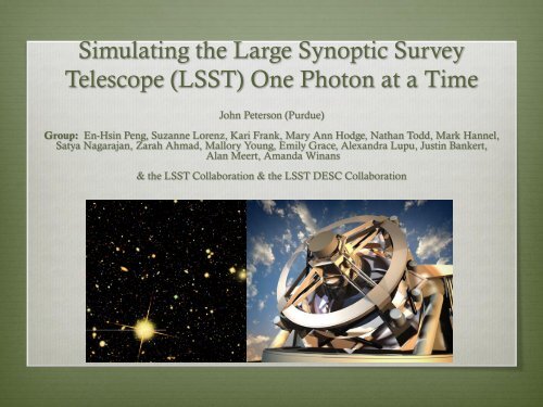
Simulating the Large Synoptic Survey<br />
Telescope (LSST) One Photon at a Time<br />
John Peterson (Purdue)<br />
Group: En-Hsin Peng, Suzanne Lorenz, Kari Frank, Mary Ann Hodge, Nathan Todd, Mark Hannel,<br />
Satya Nagarajan, Zarah Ahmad, Mallory Young, Emily Grace, Alexandra Lupu, Justin Bankert,<br />
Alan Meert, Amanda Winans<br />
& the LSST Collaboration & the LSST DESC Collaboration
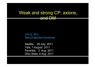
Most measurements<br />
have suggested a<br />
<strong>Universe</strong> of mostly dark<br />
energy, some dark<br />
matter, and little baryon<br />
filled <strong>Universe</strong><br />
CMB ~ total content:<br />
few % within critical<br />
Clusters ~ DM/atoms<br />
ratio is ~6<br />
Supernovae~DE<br />
dominant in expansion<br />
BBN ~ small fraction of<br />
atoms<br />
Modern Cosmology<br />
Dark<br />
Matter<br />
22%<br />
Atoms<br />
4%<br />
Dark<br />
Energy<br />
74%<br />
Is this even right? 96% of the <strong>Universe</strong> is beyond<br />
the Standard Model. What is the consequence of<br />
this? What can we measure about these further?
Future Measurements in Cosmology<br />
Need more data to get higher statistical precision<br />
Need multiple astrophysical techniques<br />
However, when you push towards higher statistical<br />
precision have new systematics that need to be<br />
understood<br />
And with a large enough quantity of data & high<br />
enough precision would need both fast and high<br />
fidelity simulations to understand these details
High Precision Cosmological Techniques<br />
1) SNe to Measure Expansion Rate<br />
(Perlmutter 1998; Reiss 1998)<br />
2) Time delays in strong lens images<br />
(Suyu 2010)<br />
3) Cluster Mass Function Evolution<br />
(Vikhlinin 2009; JRP 2012)<br />
Growth of Structure (e.g. Springel 2005)<br />
4) Baryon<br />
Acoustic<br />
Oscillations in<br />
Matter Power<br />
Spectrum<br />
(Eisenstein 2005)
5) Weak Gravitational Lensing<br />
High Precision Cosmological Techniques<br />
Knox et. al 2004
High Precision Cosmological Techniques<br />
Hu 2008<br />
Dark Energy Constraints<br />
Will have increasing<br />
discriminatory power<br />
to distinguish between<br />
cosmological constant<br />
and various models<br />
LSST will measure:<br />
3 billion galaxies<br />
10 billion stars<br />
1 million SNe<br />
10,000 clusters<br />
Dark Matter Map<br />
of Entire Sky<br />
[Also the other major area requiring high precision is stellar astrometry where large<br />
Fraction of milky way will be mapped with proper motions & some parallaxes]
How does LSST do this? Etendue<br />
Etendue is the product of<br />
Area and Field of View<br />
To get more area simply build<br />
a large telescope<br />
To get higher field of view, favor<br />
designs with shorter focal lengths,<br />
and minimal vignetting, reasonable<br />
off-axis image quality<br />
Consequence of this is have to<br />
build a large camera<br />
Consequence of a large camera is<br />
large data rate
Large Synoptic Survey Telescope (LSST)<br />
Adler Planetarium, Brookhaven National Laboratory (BNL), California Institute<br />
of Technology, Carnegie Mellon University, Chile, Cornell University, Drexel<br />
University, Fermi National Accelerator Laboratory, George Mason University,<br />
Google, Inc., Harvard-Smithsonian Center for Astrophysics, Institut de Physique<br />
Nucleaire et de Physique des Particules (IN2P3), Johns Hopkins University,<br />
Stanford University, Las Cumbres Observatory Global Telescope Network, Inc.,<br />
Lawrence Livermore National Laboratory (LLNL), Los Alamos National<br />
Laboratory (LANL), National Optical Astronomy Observatory, Princeton<br />
University, Purdue University, Research Corporation for Science Advancement,<br />
Rutgers University, SLAC National Accelerator Laboratory, Space Telescope<br />
Science Institute, Texas A & M University, The Pennsylvania State University,<br />
University of Arizona, University of California at Davis, University of California<br />
at Irvine, University of Illinois at Urbana-Champaign, University of Michigan,<br />
University of Pennsylvania, University of Pittsburgh, University of Washington,<br />
Vanderbilt University<br />
Largest survey telescope: Highest Etendue (area*FOV)<br />
for a telescope: 320 m2deg2 www.lsst.org<br />
Largest data rate 10Tb/night!<br />
8.4 m mirror; 6 filters (300-1100 nm)<br />
Largest Astronomical Camera<br />
Joint NSF & DoE project<br />
Commissioning in ~2019;<br />
First science observations in ~2021<br />
Surveys the ½ the sky every few nights<br />
Get ~1000 images in 6 colors over 10 years to ~27 mag<br />
of everything (billions of galaxies & stars, & all<br />
asteroids >150 m, rare objects)
LSST Site
LSST Mirrors
LSST Camera
Importance of Simulations for LSST<br />
More data than any other astronomical project<br />
Produces 3 gigapixel images (~1500 HDTV’s) every 15<br />
seconds<br />
No one can ever look at all the data Automatic<br />
processing (that has to work when telescope turns on)<br />
In addition, some of the most accurate measurements ever<br />
made have been planned especially for cosmology<br />
Maybe we should do some simulations<br />
Have led development of a novel photon simulation<br />
(phoSim) code for several years in the LSST project
COSMO-<br />
LOGICAL<br />
SIMULATOR:<br />
Synthetic<br />
<strong>Universe</strong> is<br />
constructed<br />
DESC Simulation & Analysis Framework<br />
object 0.002 -<br />
2.439485 14.5<br />
galaxySED/Const64e<br />
0804z..spec.gz 0 0 0<br />
0 0 0 sersic2D<br />
1.29394 2.4587 1.77<br />
2.980 ccm 2.3 8.2<br />
ccm 2.78 9.45<br />
<strong>Universe</strong> Catalogs Photons Images <br />
Measurements<br />
CATALOG<br />
CONSTRUCTOR<br />
(CATSIM):<br />
<strong>Universe</strong> is<br />
parameterized<br />
in catalogs that<br />
can later be<br />
photon sampled<br />
PHOTON SIMULATOR<br />
(PHOSIM):<br />
Atmosphere,<br />
Telescope, &<br />
Camera physics<br />
formulated in terms<br />
of photon<br />
manipulations<br />
Image Simulations (IMSIM)=PHOSIM+CATSIM<br />
w=-1.00000<br />
+/- 0.00001<br />
DATA<br />
MANAGEMENT (DM) &<br />
DESC LEVEL-3<br />
ANALYSIS:<br />
Image processing to<br />
produce catalogs and<br />
measurements<br />
on the catalogs<br />
14
First order image properties<br />
Photometric zeropoint<br />
Background level<br />
PSF size<br />
Astrometric scale<br />
Image Properties<br />
Some existing simulators (Sky Maker (Bertin),<br />
Shapelets (Dobke), GalFast (Mandelbaum),<br />
DES (Lin)) use parametric models to capture<br />
some image properties<br />
To get detailed second image properties have<br />
to go to full photon Monte Carlo approach<br />
Essentially all DE measurements depend on<br />
some combination of detailed PSF<br />
size/shape, astrometry, or photometry<br />
Second Order Image properties<br />
PSF size wavelength dependence<br />
PSF size spatial dependence<br />
PSF size spatial variation<br />
PSF shape (ellipticity and other moments)<br />
PSF wings<br />
PSF shape wavelength-dependence<br />
PSF shape spatial decorrelation<br />
PSF shape spatial variation<br />
Differential astrometric non-linearity<br />
Differential astrometric wavelength-dependence<br />
Differential astrometric decorrelation<br />
Photometric chromaticity<br />
Photometric variation in time<br />
Background spatial dependence<br />
Background spatial variation<br />
Background wavelength dependence<br />
And more…
Optical Photon Monte Carlo Simulations
Sky:<br />
Observing configuration from OpSim<br />
Photon Monte Carlo for Galaxies (elliptical Sersic<br />
bulge/disk), Stars, Asteroids (moves during & between<br />
exposures)<br />
Dust absorption at source & Milky Way<br />
Separate SEDs for every object<br />
Instance Catalogs to include other objects<br />
Background of blank sky, moon, twilight, inc. gradients<br />
Atmosphere:<br />
Multi-layer multi-scale frozen Kolmogorov screens<br />
Outer scale model<br />
Seasonal Wind model for LSST site<br />
Turbulence vs. height model for LSST site<br />
Atmospheric raytrace (refractive turbulence & optical<br />
depth)<br />
Atmospheric dispersion<br />
Atmospheric molecular opacity (wavelength, height, &<br />
time dependent)<br />
Multi-level grey cloud model<br />
Physics of PhoSim<br />
Optics & Detector:<br />
Reflection/Refraction in optics/detector<br />
Diffraction<br />
LSST Optics Design (filter-dependent)<br />
Focal plane layout<br />
Two-level Spider design<br />
Alt/Az Tracking Errors, Rotation Jitter, Spider rotation<br />
Dome Seeing<br />
Surface Perturbations & Alignment errors of<br />
mirrors/lenses/detectors<br />
Large Angle Scattering<br />
Angle-dependent filter curves<br />
Lens coatings<br />
Mirror Reflectivity<br />
Saturation & Blooming<br />
Detector A/R<br />
QE & Charge diffusion model<br />
Cosmic rays<br />
Read Noise, Dark Current, Gain, Pre-scans, Offsets<br />
for amplifiers<br />
Hot pixels/columns & dead pixels<br />
Non-uniform QE Maps<br />
CTE<br />
Biases/Darks/Flats<br />
Complete Optimization for saturation, background, photon removal,<br />
& non-sequential rays<br />
17
Very important physics<br />
PSF size, shape, & astrometry (where the photon lands)<br />
Optical Design<br />
Perturbations/Misalignments<br />
Charge Diffusion<br />
Turbulence<br />
Photometry (how many photons)<br />
Geometric design<br />
Rayleigh scattering<br />
Filter multi-layer coatings<br />
Photo-electric conversion<br />
18
Regimes of<br />
Image Simulation<br />
Aberrations+Diffusion<br />
>> λ(f/#)<br />
Aberrations+Diffusion<br />
r 0~10 cm<br />
D > r 0~ 10cm<br />
D D/v ~ .1s<br />
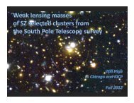
Modern Survey Telescopes
Monte Carlo Efficiency<br />
Basically doing a Monte Carlo over the incident radiation field through<br />
Time-dependent & Wavelength-dependent Physics<br />
Extremely fast way of doing this integral even if we have large numbers of photons
PhoSim<br />
Architecture<br />
Static Physics & Design Data<br />
SEDs of <strong>Universe</strong>,<br />
sky background/moon data<br />
LSST camera, telescope, &<br />
site specific files<br />
Cosmic ray templates,<br />
Earth-specific atmosphere data<br />
Code<br />
Data<br />
User<br />
User<br />
Integration<br />
Validation<br />
Tests<br />
Loop over visits<br />
Instance Catalog<br />
Operation<br />
Commands<br />
Astro<br />
Catalog<br />
Physics<br />
command<br />
override files<br />
(optional)<br />
Loop over chips<br />
Trim<br />
PhoSim<br />
script<br />
Photon<br />
Raytrace<br />
Instrument<br />
Config<br />
Extra Outputs:<br />
eimage<br />
Centroid files<br />
Surface throughput<br />
files<br />
Event files<br />
Atmosphere<br />
Creator<br />
Electron<br />
->ADC<br />
Loop over<br />
exposures<br />
Amplifier<br />
images
Catalog Constructor<br />
Connolly, Krughoff, Gibson (UW)<br />
A catalog of positions, motions (proper motions, orbits), and<br />
physical properties (types, SEDs, spatial model, etc.) of<br />
objects expected to be seen by LSST.<br />
It is a multi-billion row relational database, and a suite of<br />
Python tools.<br />
Used to create “instance catalogs” what is in the sky at<br />
a given time and what are their spatial & spectral properties;<br />
Include operational data of environment and observation<br />
control (moon position, filter, exposure, etc.)<br />
LSST Operation Simulator
Galaxies from ΛCDM N-Body Simulations: Galaxy positions and properties from<br />
Millennium N-body simulation catalogs with gas cooling, star formation,<br />
supernovae and AGN (Lucia et al. 2008); Up to 28 mag in r-band/23 million galaxies<br />
Morphologies modeled with combination of Sérsic profiles – ellipticals and bulge +<br />
disk (Lucia et al., Gonzalez et al.); Spectral Energy Distribution fit to colors of source using<br />
spectral models (Bruzual & Charlot)<br />
Milky Way model of 10 million detectable stars; Based on state-of-the-art Galactic<br />
structure models surveys (Juric et al. (2008), Ivezic et al. (2008), Bond et al. (2010), Sesar, Juric and Ivezic<br />
(2011), Lopez-Corredoira et al. (2005)); Includes a full three-dimensional Interstellar dust<br />
distribution model to redden SEDs of stars & galaxies (Amores & Lepine (2005), matched to<br />
Schlegel, Finkbeiner, Davis (1998) maps at infinity)<br />
10.6 M object Solar System Model w/ orbits & obs. Properties: inclues Near Earth<br />
Objects,Main Belt Asteroids, Trojans, Trans-Neptunian Objects, Scattered Disk<br />
Objects, (PanSTARRS Model, PASP 123, 423 (2011),Bottke et al 2002, Morbidelli et al, Grav et al. 2011)<br />
Variable stars and transient objects (e.g. SNe)<br />
r-i (mag)<br />
CatSim<br />
g-r (mag) g-r (mag)<br />
SDSS
Draw Photons<br />
Direction: Direction chosen by (ra, dec) and telescope pointing<br />
(ra,dec) & rotator angle<br />
Wavelength: Monte Carlo Sample SED files to choose<br />
wavelength in rest frame of source<br />
Time: Monte Carlo Sample time between start and stop of<br />
exposure<br />
Position: Start at the top of the atmosphere in pupil pattern<br />
Additional Astrophysics:<br />
Redshift: photon has wavelength redshifted after drawing from rest frame<br />
Dust: Two dust models that destroy the photons according to reddening laws; Apply both in<br />
the rest frame for internal reddening & in our frame from Milky Way models<br />
Lensing: Extended source models can be distorted by measuring their position from the center<br />
of the source and distorting final position of photon according to γ1 and γ2 24
Kolmogorov~k -11/3<br />
r 0<br />
Outer Scale<br />
Aperture size<br />
Atmosphere Turbulence<br />
Phase screens<br />
Temperature fluctuation in the<br />
atmosphere cause index of refraction<br />
variations and result in “seeing”<br />
Well-known that atmospheric<br />
turbulence has approximately<br />
Kolmogorov spectrum (k -11/3 ) up to<br />
outer scale L 0 (von Karman)<br />
These patterns are essentially frozen<br />
and drift with constant velocity in a<br />
series of layers (Taylor)
Atmosphere Model<br />
Photons accumulate<br />
Refractive kicks through<br />
Frozen drifted phase screens<br />
of turbulence;<br />
Possibly lost due to opacity<br />
Diffraction on scales below 2 r 0<br />
treated by full diffraction calculation<br />
Atmospheric Dispersion simulated
Atmosphere Structure<br />
Wind model (direction & data) uses data<br />
based on seasonal monthly averages for<br />
LSST latitude and longitude<br />
Model for turbulence intensity as a<br />
Function of height<br />
Model for outer scale a function of height
Atmosphere Opacity<br />
1) Cloud model<br />
2) Molecular opacity<br />
O 3<br />
O 2<br />
H 2O<br />
3) Rayleigh scattering<br />
4) Aerosols<br />
Have complex spatial & temporal variation<br />
Local optical depth calculated for each ray<br />
segment<br />
Absorption is pressure-dependent and therefore<br />
height dependent
Star Grids<br />
29
Raytracing through<br />
Telescope & Camera Optics<br />
Series of optical surfaces (2D)<br />
that divide the 3-D volume into<br />
different media (glass, silicon, air)<br />
Ray intercepts are found by<br />
minimizing the distance between the<br />
end of the ray and the surface<br />
Interactions can occur at interfaces<br />
(reflection, refraction, absorption)
Each filter configuration has every surface<br />
defined by the asphere equation<br />
Each surface specifies the media (silicon, glass, air) between the surface<br />
in the 3-D volume<br />
Chips in detector plane specified by rectangular surfaces having a<br />
nominal center, pixel size, x & y sizes<br />
Name Type R curv Δz r out r in κ α 3 α 4<br />
Optical Elements<br />
α 5<br />
α 6<br />
α 7<br />
α 8<br />
α 9<br />
α 10<br />
Coating Medium<br />
M1 Mirror 19835 0 4180 2558 -1.215 0 0 0 1.381e-27 0 0 0 0 Mirror Vacuum<br />
M2 Mirror 6788 6156.2 1710 900 -0.222 0 0 0 -1.274e-23 0 -9.68e-<br />
31<br />
M3 Mirror 8344.5 -6390 2508 550 0.155 0 0 0 -4.5e-25 0 -8.15e-<br />
33<br />
0 0 Mirror Vacuum<br />
0 0 Mirror Vacuum<br />
None None 0 3630.5 0 0 0 0 0 0 0 0 0 0 0 None Vacuum<br />
L1 Lens 2824 34.568418 775 0 0 0 0 0 0 0 0 0 0 Lens A/R Glass<br />
L1E Lens 5021 82.23 775 0 0 0 0 0 0 0 0 0 0 Lens A/R Vacuum<br />
L2 Lens 0 412.64202 551 0 0 0 0 0 0 0 0 0 Lens A/R Glass<br />
L2E lens 2529 30 551 0 -1.57 0 0 1.656e-21 0 0 0 0 Lens A/R Vacuum<br />
F filter 5632 349.58 378 0 0 0 0 0 0 0 0 0 Filter 0 Glass<br />
FE filter 5530 26.60 378 0 0 0 0 0 0 0 0 0 None Vacuum<br />
L3 lens 3169 42.40 361 0 -0.962 0 0 0 0 0 0 0 Lens A/R Glass<br />
L3E lens -13360 60 361 0 0 0 0 0 0 0 0 0 Lens A/R Vacuum<br />
31
Every optical surface & CCD has an ideal location<br />
Perturbations,<br />
Misalignments,<br />
& Tracking Errors<br />
During a particular simulation all surfaces & CCDs can be misaligned by the 6<br />
degrees of freedom; Each optical surface can also have a surface perturbations<br />
place on the surface that represent the deviation from the ideal shape<br />
These represent the perturbations & misalignments induced by the thermal,<br />
vibrational, pressure, gravitational stresses while the telescope is operating with<br />
the full control system as well as fabrication errors<br />
In general, the perturbations & misalignments tend to induce anisotropic PSFs<br />
that are highly correlated across the entire focal plane (because mostly in pupil<br />
plane)<br />
Also have tracking model for perturbations during an exposure<br />
dxi = fiu ¥ + dxi dT T -T ( 0 +dTgT ) + dxi dq q +dqg ( m)<br />
+ hig0 + Aij ( aj +da jga )<br />
-1 -1<br />
aj = Aji Pi + Ajl Zlk<br />
æ<br />
ç<br />
è<br />
-1 ak ç<br />
1+<br />
Navg ö<br />
g ÷<br />
0 ÷<br />
ø<br />
ZkiUi
Multilayer Coatings<br />
Photons reflected or transmitted<br />
according to multilayer models<br />
which are angle and wavelength<br />
dependent<br />
Photoelectron Conversion<br />
Photons can convert into electrons<br />
as they traverse the Silicon<br />
(temperature-dependent)
After 1 micron<br />
After 10 microns<br />
Rasmussen<br />
After 100 microns<br />
After 50 microns After 300 microns<br />
Electron Diffusion<br />
First, electric field profile as a function of<br />
height is calculated (voltage & dopant density<br />
model dependent)<br />
Then electron is drifted in segments and lateral<br />
diffusion is set by local diffusion constant;<br />
Leads to non-gaussian profile
Other Effects<br />
Spider diffraction<br />
Dome seeing<br />
Large angle scattering from mirror<br />
micro-roughness & Mie scattering<br />
Bleeding & Saturation<br />
Ghosts<br />
Cosmic Rays
Background Model<br />
Two components:<br />
Air glow & scattered<br />
Moonlight<br />
Moon has Mie scattering &<br />
Rayleigh scattering which<br />
leads to color-dependent<br />
spatial gradient<br />
Airglow has spatial<br />
variation & temporal<br />
variation<br />
Adams et al.
Digitization<br />
Amplifier Segmentation<br />
CTE (one electron at a time)<br />
Pre/Over scans<br />
ADC using bias, gain, nonlinearity<br />
model with variation<br />
Bit error in ADC<br />
Dark current<br />
Read noise & variation<br />
Hot pixels<br />
Hot columns<br />
Dead Pixels<br />
PRNU
0.2”<br />
Optics +Tracking +Diffraction +Det Perturbations<br />
+Lens Perturbations +Mirror Perturbations +Detector +Dome Seeing<br />
+Low Altitude +Mid Altitude +High Altitude +Pixelization<br />
Atmosphere Atmosphere Atmosphere<br />
38
0.2”<br />
Optics +Tracking +Diffraction +Det Perturbations<br />
+Lens Perturbations +Mirror Perturbations +Detector +Dome Seeing<br />
+Low Altitude +Mid Altitude +High Altitude +Pixelization<br />
Atmosphere Atmosphere Atmosphere 39
Entire<br />
focal plane<br />
3<br />
gigapixels<br />
1000 CPU<br />
hours<br />
1 trillion<br />
photons<br />
Done on<br />
grid<br />
computing
Central<br />
5 x 5 chips<br />
~1 sq. degree<br />
41
Central chip<br />
15’ x 15’<br />
42
ImSim Description 44
ImSim Description 45
3 Color<br />
Image
4 Major LSST Data Challenges so far (4/09,6/10,9/10,5/11,4/12); Run on grid computing at Purdue<br />
(incl. OSG), UW, SLAC, and Google; Currently produce data at ~10% of real time; All analyzed by<br />
Data Management Pipelines<br />
4 thousand visits<br />
28 million amplifier images<br />
44 billion astrophysical objects<br />
4 quadrillion photons<br />
Photometry<br />
Everything<br />
compared to<br />
simulation truth<br />
(not possible<br />
with real data)<br />
Astrometry Completeness PSF size & shape
JRP, Bard, Allen, Li, Cui<br />
Blind shear survey with 10 sq. degrees<br />
Estimated shear systematic floor<br />
Chang et al. 2012
Validation!
Conclusions<br />
Have a multi-purpose high fidelity optical image<br />
simulator (PhoSim) with physics appropriate for<br />
optical survey telescopes<br />
Will enable a number of state-of-the art algorithms to<br />
be developed that necessary for high precision<br />
cosmological measurements in the LSST DESC<br />
LSST will enable dark energy properties to be<br />
measured in unprecented detail & will make dark<br />
matter map of the entire sky<br />
Also possible to use for other telescopes