12-02-Cahier-R- ... e-Chevallier-Gastineau.pdf - Base ...
12-02-Cahier-R- ... e-Chevallier-Gastineau.pdf - Base ...
12-02-Cahier-R- ... e-Chevallier-Gastineau.pdf - Base ...

You also want an ePaper? Increase the reach of your titles
YUMPU automatically turns print PDFs into web optimized ePapers that Google loves.
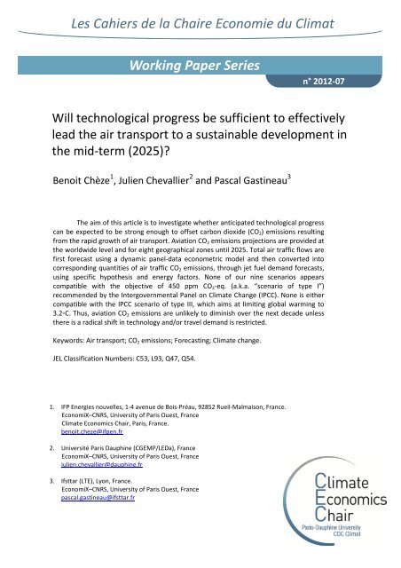
Les <strong>Cahier</strong>s de la Chaire Economie du Climat<br />
Working Paper Series<br />
Will technological progress be sufficient to effectively<br />
lead the air transport to a sustainable development in<br />
the mid-term (2<strong>02</strong>5)?<br />
approach<br />
Benoit Chèze 1 , Julien <strong>Chevallier</strong> 2 and Pascal <strong>Gastineau</strong> 3<br />
The aim of this article is to investigate whether anticipated technological progress<br />
can be expected to be strong enough to offset carbon dioxide (CO2) emissions resulting<br />
from the rapid growth of air transport. Aviation CO2 emissions projections are provided at<br />
the worldwide level and for eight geographical zones until 2<strong>02</strong>5. Total air traffic flows are<br />
first forecast using a dynamic panel-data econometric model and then converted into<br />
corresponding quantities of air traffic CO2 emissions, through jet fuel demand forecasts,<br />
using specific hypothesis and energy factors. None of our nine scenarios appears<br />
compatible with the objective of 450 ppm CO2-eq. (a.k.a. “scenario of type I”)<br />
recommended by the Intergovernmental Panel on Climate Change (IPCC). None is either<br />
compatible with the IPCC scenario of type III, which aims at limiting global warming to<br />
3.2◦C. Thus, aviation CO2 emissions are unlikely to diminish over the next decade unless<br />
there is a radical shift in technology and/or travel demand is restricted.<br />
Keywords: Air transport; CO2 emissions; Forecasting; Climate change.<br />
JEL Classification Numbers: C53, L93, Q47, Q54.<br />
1. IFP Energies nouvelles, 1-4 avenue de Bois-Préau, 92852 Rueil-Malmaison, France.<br />
EconomiX–CNRS, University of Paris Ouest, France<br />
Climate Economics Chair, Paris, France.<br />
benoit.cheze@ifpen.fr<br />
2. Université Paris Dauphine (CGEMP/LEDa), France<br />
EconomiX–CNRS, University of Paris Ouest, France<br />
julien.chevallier@dauphine.fr<br />
3. Ifsttar (LTE), Lyon, France.<br />
EconomiX–CNRS, University of Paris Ouest, France<br />
pascal.gastineau@ifsttar.fr<br />
n° 20<strong>12</strong>-07
Will technological progress be sufficient to effectively<br />
lead the air transport to a sustainable development in<br />
the mid-term (2<strong>02</strong>5)? ∗<br />
Benoît Chèze † ‡ § , Julien <strong>Chevallier</strong> ‡ ‡<br />
, and Pascal <strong>Gastineau</strong><br />
April <strong>12</strong>, 20<strong>12</strong><br />
Abstract<br />
The aim of this article is to investigate whether anticipated technological progress<br />
can be expected to be strong enough to offset carbon dioxide (CO2) emissions resulting<br />
from the rapid growth of air transport. Aviation CO2 emissions projections are provided<br />
at the worldwide level and for eight geographical zones until 2<strong>02</strong>5. Total air traffic flows<br />
are first forecast using a dynamic panel-data econometric model and then converted into<br />
corresponding quantities of air traffic CO2 emissions, through jet fuel demand forecasts,<br />
using specific hypothesis and energy factors. None of our nine scenarios appears com-<br />
patible with the objective of 450 ppm CO2-eq. (a.k.a. “scenario of type I”) recommended<br />
by the Intergovernmental Panel on Climate Change (IPCC). None is either compatible<br />
with the IPCC scenario of type III, which aims at limiting global warming to 3.2 ◦ C.<br />
Thus, aviation CO2 emissions are unlikely to diminish over the next decade unless there<br />
is a radical shift in technology and/or travel demand is restricted.<br />
Keywords: Air transport; CO2 emissions; Forecasting; Climate change.<br />
JEL Classification Numbers: C53, L93, Q47, Q54.<br />
∗ The authors are grateful to the Lunch-Seminar’s participants (2011, April) of the Economics Department<br />
of IFP Energies nouvelles (IFPEN). The authors also thank for their helpful comments L. Meunier (ADEME)<br />
and from the IFPEN: E. Bertout, P. Coussy, P. Marion, A. Pierru, J. Sabathier, V. Saint-Antonin, S. Tchung-<br />
Ming and S. Vinot. The usual disclaimer applies.<br />
† Corresponding author. IFP Energies nouvelles, 1-4 avenue de Bois-Préau, 92852 Rueil-Malmaison, France.<br />
benoit.cheze@ifpen.fr.<br />
‡ EconomiX–CNRS, University of Paris Ouest, France.<br />
§ Climate Economics Chair, Paris, France.<br />
Université Paris Dauphine (CGEMP/LEDa), France; julien.chevallier@dauphine.fr.<br />
Ifsttar (LTE), Lyon, France; pascal.gastineau@ifsttar.fr.<br />
1
1 Introduction<br />
This article proposes a discussion about the future evolution, until 2<strong>02</strong>5, of carbon dioxide<br />
(CO2) emissions from the air transport sector. Besides, it analyses whether technological<br />
progress would be sufficient to outweigh growth in fuel use, and lead to either absolute or<br />
even relative CO2 emission reductions. As shown in Figure 1, the share of CO2 emissions com-<br />
ing from air transport in total CO2 emissions linked to burning fossil fuels has been increasing<br />
from 2% in 1980 to 2.5–2.7% in 2007, i.e. an increase by 25% in less than thirty years. This<br />
evolution seems to have slowed down during the last decade (Figure 1 (a)). However, this<br />
slower pace cannot be associated with decreasing CO2 emissions coming from air transport,<br />
which have been steadily increasing from 350 Mt in 1980 to 750 Mt in 2007. Instead, it is due<br />
to an even stronger increase of the total CO2 emissions linked to burning fossil fuels (Figure<br />
1 (b)).<br />
Share of CO2 emissions from air<br />
transport in total CO2 emissions<br />
3.0<br />
2.5<br />
2.0<br />
1.5<br />
1.0<br />
0.5<br />
0<br />
1980 1984 1988 1992 1996 2000 2004<br />
Total CO2 emissions linked<br />
to burning fossil fuels (Mt)<br />
30000<br />
25000<br />
20000<br />
15000<br />
10000<br />
5000<br />
0<br />
1980 1984 1988 1992 1996 2000 2004<br />
fossil fuels<br />
(a) (b)<br />
air transport<br />
Figure 1: Evolution of the share of CO2 emissions coming from air transport in total CO2<br />
emissions linked to burning fossil fuels (graph (a)) as well as CO2 emissions coming from air<br />
transport (graph (b), right axis) and total CO2 emissions linked to burning fossil fuels (graph<br />
(b), left axis) from 1980 to 2007.<br />
Source: Authors, from IEA data.<br />
As a first conclusion, and even if Figure 1 does not take into account all greenhouse gases<br />
(GHG) emissions 1 , the current contribution of the air transport sector to climate change may<br />
1 CO2 is one of the six gases whose anthropic origin is recognized by the UN Framework Convention on<br />
Climate Change adopted by the Rio Summit in 1992. Other greenhouse gases include CH4, N2O, and fluorized<br />
gases (HFC, PFC, SF6).<br />
2<br />
2000<br />
1000<br />
0<br />
CO2 emissions from<br />
air transport (Mt)
e seem as quite marginal. This statement shall not be misleading, and yield to undermine<br />
the risks associated with a continuous growth of the demand for air transport in the near<br />
future. At least for two reasons. First, Figure 1 shows only the CO2 emissions coming from<br />
air transport. There are other greenhouse gases associated with this activity, such as H2O<br />
and NOX, which have important climatic impacts 2 . Second, it is not negligible if we include<br />
the environmental risk attached to a sustained growth for the demand in air transport, which<br />
urges to take action. This sector indeed is growing very quickly, and the share of its emissions<br />
is steadily increasing (Figure 1). In 1999, the special report on air transport by the IPCC<br />
estimated that this sector could be characterized by a growth of its CO2 emissions comprised<br />
between 60% and more than 1000% from 1992 to 2050 (IPCC, 1999). Along with increasing<br />
environmental pressures, this future development of the aviation sector may be seen as un-<br />
sustainable.<br />
That is why policy makers are more and more concerned by the future evolution of air<br />
transport, especially in Europe, and aim at limiting its CO2 emissions (Rothengatter, 2010,<br />
Zhang et al., 2010). Against this background, the international climate negotiations aim at<br />
reducing GHG emissions as much as possible, and compatible with the objective of limiting<br />
global warming by +2 ◦ C (degrees Celsius) compared to the pre-industrial era 3 . To comply<br />
with this objective, the EU Commission has established in April 2009 the target to reduce<br />
greenhouse gases emissions by 20% in 2<strong>02</strong>0 in its “Energy-Climate” Package. These reduction<br />
objectives are binding, and will also concern civil aviation with its inclusion in the EU ETS 4 .<br />
To sum up, policy makers distinguish between two kinds of measures to limit the environ-<br />
2 For instance, H2O and NOX emissions produce ozone. The Intergovernmental Panel on Climate Change<br />
(IPCC, 1999) estimates that these gases represent between 50% and 80% of the potential of global warming<br />
linked to aviation. However, these gases are difficult to quantify, since they vary depending on the type of<br />
flight. Besides, by their very nature (such as NOX which are indirect gases for instance), their impacts on the<br />
climate depend on the location and the length of the emissions, and are not well understood by the scientific<br />
community to date. The IPCC therefore cautiously multiplies by a factor of two the CO2 emissions coming<br />
from air transport in order to account for the total CO2 emissions of this sector, which are then expressed in<br />
CO2 equivalent gases (CO2-eq.).<br />
3 Since the Copenhagen COP/MOP Meeting in December 2009, the scientific objective has indeed been set<br />
to +2 ◦ C. Recall that to achieve this +2 ◦ C target of limiting global warming, the IPCC suggests to decrease<br />
GHG emissions in industrialized countries by 25% to 40% in 2<strong>02</strong>0, and by 80% to 95% in 2050 compared to<br />
1990 levels (IPCC, 2007a, 2007b, SEG, 2007).<br />
4 As of 20<strong>12</strong>, airline companies traveling in the EU must limit their CO2 emissions to 97% of the annual<br />
mean recorded between 2004 and 2006. The airplanes taking off and landing in the EU 27, as well as coming<br />
from other countries, will fall under this regulation.<br />
3
mental impact of the growth of air transport. The first one consists in improving the energy<br />
efficiency of aircrafts (and thus to lower their carbon intensity) by promoting technological<br />
innovation. The second one consists in binding measures dealing with the demand for air<br />
transport 5 . These two types of measures are not antinomic and may be pursued simultane-<br />
ously. For instance, the European Commission actively promotes innovation efforts by air<br />
companies through Research & Development (R&D) programs 6 , while also taking binding<br />
actions with the inclusion of aviation in the EU ETS. However, these public policies do not<br />
follow the same logic. Indeed, the latter kind of measure deals directly with the causes of<br />
greenhouse gases emissions linked to the growth of the air transport sector, while the former<br />
kind of measure only attempts at diminishing its negative consequences.<br />
There is a sharp debate today on the best course of action to reduce significantly, and<br />
within a reasonable time horizon, greenhouse gases emissions in the air transport sector. Will<br />
technological changes 7 be sufficient to outweigh growth in fuel use? In other words, shall we<br />
solely aim at reducing the carbon intensity of the air transport sector through innovation? Or<br />
shall we admit that technological innovation alone does not allow to achieve the objectives<br />
of stablization and reduction of greenhouse gases that were set? In both cases, shall we limit<br />
the development of the air transport sector?<br />
The actors in the aeronautical industry tend to reject majoritarily the second kind of<br />
measure. For instance, concerning the inclusion of the air transport sector in the EU ETS,<br />
governments and international airlines outside Europe protest against this measure. Oppos-<br />
ing states (including Brazil, the U.S., China, and Japan) claim that the unilateral application<br />
of the EU ETS to international aviation violates the ‘cardinal principle of state sovereignty’,<br />
and assert that non-EU aircraft operators should be exempt from this trading scheme. Aero-<br />
5 To be more precise, there are actually four general types of mitigation-related measures: climate policy,<br />
behavioural change, management and new technologies. All of these, with the exception of behavioural change,<br />
are supposed to contribute to efficiency gains in the aviation sector. Behavioural change, on the other hand, is<br />
supposed to make a contribution through low carbon choices (shorter flight distances, more environmentally<br />
pro-active airlines, direct flights, etc.).<br />
6 Two main projects are devoted currently to alternative fuels (other than jet fuel) for aviation. The program<br />
Alfa-Bird, which was created in 2008 for a period of four years and coordinated by Airbus, aims at better<br />
identifying the needs in terms of research and investments. The Swafea program, lead since January 2009 by<br />
the French Aerospace Lab, aims at elaborating a roadmap for deploying alternative fuels in the mid-term.<br />
Many industrial actors (Airbus, Avio, Dassault, EADS, Rolls-Royce, Safran, Sasoil, Shell, Snecma, etc.) are<br />
participating to these programs, along with public research centers.<br />
7 Notably including the development of biofuels.<br />
4
nautical industrials argue that there have been considerable advances in the carbon intensity<br />
of aircrafts since the start of the 1990s. Arguably, energy efficiency gains due to technological<br />
progress and the enhancement of the Air Traffic Management (ATM) have largely limited the<br />
impact of the growth of the air transport sector on the growth of greenhouse gases emisssions.<br />
They claim that technological innovation through R&D expenditures should be sufficient to<br />
stabilize and then reduce greenhouse gases. For instance, the Advisory Council for Aero-<br />
nautics Research in Europe (ACARE) has announced its will to develop by 2<strong>02</strong>0 aircrafts<br />
emitting two times less CO2 emissions than aircrafts commercialized in 2000. The Interna-<br />
tional Civil Aviation Organization (ICAO) is asking its members to reduce on average by 2%<br />
per year their consumption of jet fuel until 2<strong>02</strong>0. The International Air Transport Association<br />
(IATA), which concentrates 90% of airline companies, has declared that it will enhance the<br />
energy efficiency of its aircraft fleet by 25% in 2<strong>02</strong>0, i.e. by 1.5% per year on average. To<br />
meet these objectives, airline companies advocate that many technological options exist in the<br />
near future such as lighter aircrafts, enhanced design, enhanced engines’ consumption, better<br />
traffic management, and replacing jet fuel with alternative fuels (bio-fuels) up to 10% in 2017.<br />
This article aims at evaluating whether the solutions proposed by the air transport indus-<br />
try can adequately reduce the GHG emissions coming from this sector. To do so, forecasts of<br />
CO2 emissions from the air transport sector are performed based on various scenarios of evolu-<br />
tion of the energy efficiency of aircrafts (and others). We propose to examine more especially<br />
whether only technological innovation is able to effectively reduce the impact of air traffic on<br />
the growth of greenhouse gases. Technological innovation appears indeed central to tackle<br />
this environmental challenge. Arguably, the reduction of the carbon intensity of the fleet has<br />
strongly contributed to limit the impact of the growth in the air transport sector in terms of<br />
CO2 emissions. However, these emissions have been steadily increasing over the last thirty<br />
years (see Figure 1). Besides, we may observe that the growth of air transport has always been<br />
higher than energy efficiency gains over the last thirty years, so that CO2 emissions associated<br />
with this sector have also increased overtime. Despite the ambitious objectives in terms of<br />
energy efficiency gains put forward by the main stakeholders in the aviation industry, it is<br />
not straightforward that technological innovation alone will be able to annihilate the adverse<br />
environmental impacts of air transport. Evaluating whether the industrial policy proposed<br />
by the aviation industry will be enough to stabilize GHG emissions constitutes an important<br />
step to guide decision making in the public policy process. At the European level, such an<br />
evaluation is a pre-requisite to develop a coherent environmental policy in terms of reducing<br />
GHG emissions. If the current policies do not appear as sufficient, then additional binding<br />
5
measures such as the inclusion of the air transport sector in the EU ETS since january 20<strong>12</strong><br />
would appear well-founded despite the claims by aeronautical industry 8 .<br />
The analysis proceeds in two parts. Various projections of CO2 emissions in the air<br />
transport sector are presented (Section 2) and then compared with the literature (Section 3).<br />
The CO2 emissions projections presented below are deduced from forecasts of jet fuel demand<br />
presented in Chèze et al. (2011) 9 . Compared to the latter paper, the present article goes one<br />
step further by providing original projections of CO2 emissions in the air transport sector. It<br />
allows then to investigate whether or not technological innovation would be sufficient to lead<br />
to CO2 emission reductions based on various robustness checks.<br />
Section 2 details our benchmark scenario, along with a sensitivity analysis based on eight<br />
alternative scenarios. The general methodology followed in Section 2 may be summarized into<br />
three steps. First, total air traffic flows (freight + passengers) and their growth rates (per<br />
year) have to be forecast by using dynamic panel-data econometric models. Second, these air<br />
traffic forecasts are converted into corresponding quantities of jet fuel using specific energy<br />
coefficients and traffic efficiency improvements hypothesis. Third, air traffic CO2 emissions<br />
are directly deduced from jet fuel demand forecasts by using the energy factor mentioned<br />
above (one kilogram of jet fuel – Jet-A1 or Jet-A – consumed emits 3.156 kilograms of CO2,<br />
recall footnote n ◦ 9). According to our benchmark scenario (sc. A.1., see Figure 4), air traffic<br />
CO2 emissions should rise at a mean yearly growth rate of 1.9%. Driven by gross domestic<br />
product (GDP) growth, air traffic should sharply increase (4.7%/year), along with the asso-<br />
ciated demand for jet fuel (by taking into account energy efficiency improvements). Besides,<br />
none of the scenarios anticipates a decrease, or even a stabilization, of CO2 emissions in the air<br />
transport sector by 2<strong>02</strong>5 (although our benchmark scenario includes strong energy efficiency<br />
gains). Section 3 first compares the results obtained with both (i) the projections obtained<br />
in the academic literature and by the aeronautical sector and (ii) the SRES scenarios by the<br />
8 The inclusion of aviation in the EU ETS ultimately aims at modifying the behaviour of economic agents.<br />
However, the current set-up of the system should not lead to absolute emission reductions, and possibly not<br />
even to relative emission reductions.<br />
9 The CO2 emissions associated with air transport are directly linked to the quantity of jet fuel used by<br />
the aircraft fleet. Once completely oxydized, one kilogram of jet fuel (Jet-A1 or Jet-A) consumed emits 3.156<br />
kilograms of CO2. By applying this energy factor to the quantity of jet fuel used, it is readily possible to<br />
deduce the CO2 emissions coming from the air transport sector. Note that this emissions factor is officially<br />
used by the European Commission to account for the CO2 emissions from the aviation sector towards its<br />
inclusion in the European Union Emissions Trading Scheme (EU ETS) by 20<strong>12</strong> (see Amendment C(2009)<br />
2887 completing the Directive 2009/339/CE and the Decision 2007/589/CE).<br />
6
IPCC (Nakicenovic and Swart, 2000; IPCC, 2007a, 2007b) 10 . The latter comparison aims at<br />
evaluating whether our CO2 projections concerning the air transport sector are compatible<br />
with a growth rate yielding to a maximum limit of global warming to +2 ◦ C compared to the<br />
pre-industrial era (IPCC, 2007a, 2007b). Finally, Section 4 concludes.<br />
2 World and regional air traffic CO2 emissions projections<br />
until 2<strong>02</strong>5: Benchmark scenario and sensitivity analysis<br />
This Section presents various forecasts of CO2 emissions coming from air transport by 2<strong>02</strong>5.<br />
These forecasts are deduced from preliminary forecasts of jet fuel demand presented in Chèze<br />
et al. (2011). We follow thoroughly here the methodology developed by Chèze et al. (2010),<br />
which can be summarized as follows. The amount of CO2 emitted by an airplane may be<br />
deduced directly from the quantity of jet fuel consumed. Jet fuel is only used as a fuel in the<br />
aviation sector. Consequently, the consumption of jet fuel depends very closely on the demand<br />
for mobility for this transportation means. To understand the evolution of this consumption,<br />
we must start by studying the fundamentals of air transport. This task may be decomposed<br />
into three distinct steps. First, we perform various forecasts for air traffic in the mid-term<br />
(2<strong>02</strong>5), at the world and regional levels. These forecasts are derived from the prior modeling<br />
and estimation of the relationship between air transport and its main determinants. This<br />
first step relies on econometric methods. Second, the data on air traffic are converted into<br />
corresponding quantities of jet fuel based by using energy coefficients 11 . Third, we deduce<br />
from the two preceding steps the CO2 projections for the air transport sector until 2<strong>02</strong>5. This<br />
third step is simple to compute. Indeed, carbon dioxide constitutes with water vapor the<br />
main rejection of the jet fuel combustion in the atmosphere. These emissions are directly<br />
linked to the quantity of jet fuel used, i.e. burnt in order to power an aircraft, by using the<br />
CO2 emissions factor of 3.156 (recall footnote n ◦ 9) <strong>12</strong> .<br />
Before presenting our scenarios of future evolution of air traffic CO2 emissions, this Section<br />
10 These scenarios have been developed in a special report published by the IPCC (Nakicenovic and Swart,<br />
2000) abbreviated as “Special Report on Emission Scenarios”.<br />
11 Energy coefficients – as well as their evolution through time, i.e. energy gains – constitute one of the<br />
main assumptions of this work, as explained below.<br />
<strong>12</strong> Note that using this emissions factor does not allow to estimate all emissions of greenhouse gases from<br />
the air transport sector, but only the emissions coming from carbon dioxide.<br />
7
egins by summarizing air traffic and corresponding jet fuel demand forecasts obtained by<br />
Chèze et al. (2010, 2011). Their results mostly depend on two broad hypotheses. The first<br />
one concerns the future evolution of economic activity in the various regions (estimated from<br />
regional GDP growth indicators). The second hypothesis deals with the energy efficiency<br />
coefficients that have been chosen to conduct the analysis, as well as their evolution overtime<br />
(i.e. energy efficiency gains). Thus, we present the CO2 emissions projections obtained in our<br />
benchmark scenario, and then we evaluate the robustness of these results obtained depending<br />
on these two broad hypotheses.<br />
This modeling, and the associated forecasts, are applied to eight geographical zones and<br />
at the world level (i.e. the sum of the eight regions) by specifying a dynamic model on panel<br />
data. Air traffic forecasts are computed for the following regions: Central and North America,<br />
Latin America, Europe, Russia and Commonwealth of Independent States (CIS), Africa, the<br />
Middle East, Asian countries and Oceania (except China). The eighth region is China, in<br />
order to have a specific focus on this country. By doing so, this article proposes an analysis of<br />
potential future trends of air transport CO2 emissions, both at the world and regional levels,<br />
as a simple analysis of the future yearly mean growth rates of world air traffic emissions may<br />
mask a wide heterogeneity between geographical zones.<br />
2.1 Forecasting air traffic until 2<strong>02</strong>5 . . .<br />
Air traffic projections are estimated by using econometric methods based on the historical<br />
relationship between air traffic and its main drivers (Chèze et al., 2010). Air traffic projec-<br />
tions proposed are obtained by using ICAO’s air traffic data 13 during 1980-2007. According<br />
to the literature 14 , the air traffic drivers are mainly (i) GDP growth rates, (ii) ticket prices,<br />
(iii) alternative transport modes (such as train) and (iv) some external shocks such as the<br />
September 11 th terrorist attacks in 2001. Last but not least, the magnitude of these drivers<br />
appears to depend on the maturity of the transport market: the growth rates of the domestic<br />
markets of industrialized countries are lower than those of emerging countries for instance,<br />
ceteris paribus. To take into account the latter criteria, the econometric modeling proposed<br />
13 The “Commercial Air Carriers - Traffic” database of the ICAO provides air traffic for both cargo and<br />
passenger traffic. These data are both expressed in Revenue Tonne-Kilometre (RTK), so that they can be<br />
re-aggregated together. A Revenue Tonne-Kilometre denotes one tonne of load (passengers and/or cargo)<br />
transported one kilometre.<br />
14 See in particular DfT (2009), ECI (2006), Eyers et al. (2004), Gately (1988), IPCC (1999), Macintosh and<br />
Wallace (2009), Mayor and Tol (2010), RCEP (20<strong>02</strong>), Vedantham and Oppenheimer (1994, 1998), Wickrama<br />
et al. (2003).<br />
8
y Chèze et al. (2010) is carried out by using dynamic panel-data models for the eight geo-<br />
graphical zones 15 .<br />
<strong>Base</strong>d on assumptions on the evolution of the main drivers, Chèze et al. (2010) obtain<br />
different air traffic forecasts scenarios. These air traffic forecasts rely on a crucial assumption:<br />
the future evolution of the eight geographical regions’ GDP growth rates. Their <strong>Base</strong>line air<br />
traffic forecast scenario, i.e. the “IMF GDP growth rates” scenario (see Figure 4), relies in<br />
particular on the International Monetary Fund (IMF) previsions of these GDP growth rates<br />
until 2014. Two other air traffic forecast scenarios are defined to measure the sensitivity of<br />
air traffic to changes in GDP growth rates: (i) in the “Low GDP growth rates” air traffic<br />
forecasts scenario, the IMF GDP growth rates are decreased by 10%, (ii) in the “High GDP<br />
growth rates” air traffic forecasts scenario, the IMF GDP growth rates are increased by 10%<br />
(see also Figure 4).<br />
Figure 2 provides a visual representation of the <strong>Base</strong>line air traffic forecasts scenario at<br />
the world level until 2<strong>02</strong>5 (bold line, from 2008 to 2<strong>02</strong>5) and their 95 % Interval Predic-<br />
tions 16 (dashed lines, from 2008 to 2<strong>02</strong>5). According to this scenario, this model predicts<br />
first a relatively high decrease of air traffic in 2008 and 2009 (- 3.47% between 2007 and<br />
2008) followed by the recovery of its positive evolution from 2010 to 2<strong>02</strong>5 17 . World air traffic<br />
should, overall, increase at a yearly mean growth rate of 4.7% between 2008 and 2<strong>02</strong>5, rising<br />
from 637.4 to 1391.8 billion RTK (see also Table 2). These air traffic forecasts differ from<br />
one region to another. At the regional level, RTK yearly average growth rates range from 3%<br />
per year in Central and North America to 8.2% per year in China (Table 2, first two columns).<br />
Air traffic forecasts obtained by Chèze et al. (2010) are not further commented here.<br />
These air traffic forecasts are necessary to deduce (i) the associated jet fuel demand (Chèze et<br />
al., 2011) which yields to (ii) the corresponding CO2 emissions by 2<strong>02</strong>5 (i.e. what is developed<br />
in this article). The latter step is presented in the next Section.<br />
15 The influence of the main air traffic determinants is estimated by using the Arellano-Bond estimator.<br />
GDP appears to have a positive influence on air traffic, whereas the influence of the jet-fuel price - above a<br />
given threshold - is negative. Exogenous shocks may also have a (negative) impact on air traffic growth rates.<br />
16 Variance of in-sample predicted values and forecasts are different. As is intuitive, the variance of the<br />
forecasts is higher than the variance of the predicted values. This explains the progressively increasing gap<br />
between the lower bound and the upper bound of the 95 % Interval Predictions.<br />
17 Negative GDP growth rates in 2008 and 2009 (according to IMF GDP projections) mainly explain the<br />
predicted decrease of air traffic during this period (See Chèze et al. (2010) for more details).<br />
9
10 9 RTK<br />
1800<br />
1600<br />
1400<br />
<strong>12</strong>00<br />
1000<br />
800<br />
600<br />
400<br />
200<br />
0<br />
1981 1985 1989 1993 1997 2001 2005 2009 2013 2017 2<strong>02</strong>1 2<strong>02</strong>5<br />
Blue line: ICAO data; bold line: in-sample predicted values (from 1981 to 2007) and air traffic forecasts (from<br />
2008 to 2<strong>02</strong>5); dashed lines: 95 % Interval Prediction.<br />
Figure 2: World air traffic forecasts – expressed in RTK (billions) – until 2<strong>02</strong>5 (<strong>Base</strong>line<br />
scenario).<br />
Source: Chèze et al. (2010), ICAO data.<br />
2.2 . . . and corresponding aviation CO2 emissions<br />
This Section presents various CO2 emissions scenarios of air traffic until 2<strong>02</strong>5, both at the<br />
world and regional level. Recall that these scenarios correspond to CO2 emissions from Jet-A1<br />
fuel. It is thus necessary to first obtain jet fuel demand forecasts. Once this step has been<br />
performed, one can readily deduce the amount of air traffic CO2 emissions by applying an<br />
emission factor equal to 3.156. As this last step computationally simple, it has been chosen<br />
to focus in Section 2.2.1 on the methodology and the assumptions used to obtain jet fuel<br />
demand forecasts. Then, Sections 2.2.3 and 2.2.4 will present the Benchmark scenario and a<br />
sensitivity analysis of aviation CO2 emissions, respectively.<br />
2.2.1 Energy efficiency coefficients estimates and expected energy efficiency gains<br />
in the aviation sector<br />
This Section explains how projections of air transport obtained in Section 2.1 are converted<br />
into corresponding quantities of jet fuel. This task is performed based on the specific ‘Traffic<br />
Efficiency method’ developed by the UK DTI (Department of Trade and Industry) for the<br />
10
special IPCC report on air traffic (IPCC, 1999). The idea underlying this method may be<br />
summarized as follows. An increase by 5% per year of air traffic does not imply an increase by<br />
the same magnitude of jet fuel demand, and thus corresponding CO2 emissions. Indeed, the<br />
growth of jet fuel demand following the growth of air traffic is mitigated by energy efficiency<br />
gains 18 . Energy efficiency improvements is obtained thanks to enhancements of (i) Air Traf-<br />
fic Management (ATM), (ii) existing aircrafts (changes in engines for example) and (iii) the<br />
production of more efficient aircrafts (which is linked to the rate of change of aircrafts) 19 . Be-<br />
sides, by improving their load factors, airlines hold a relatively easy way to diminish their jet<br />
fuel consumption, and thus their CO2 emissions, without achieving any technological progress.<br />
The difficulty to convert air traffic forecasts into jet fuel is due to the fact that we need<br />
adequate energy efficiency coefficients on the one hand and coherent scenarios for expected<br />
growth rates, expressed per year, of their future improvements on the other hand. The latter<br />
are used to estimate energy efficiency gains. These estimates are a central issue to obtain<br />
air traffic CO2 emissions forecasts. By applying adequate energy efficiency (EE) coefficients<br />
on historical air traffic data, one can estimate corresponding jet fuel demand and then corre-<br />
sponding CO2 emissions. Second, the expected growth rates of energy efficiency coefficients<br />
(corresponding to the hypothesis of energy efficiency gains) are required to convert air traf-<br />
fic forecasts into projections of (i) corresponding jet fuel demand, and then (ii) CO2 emissions.<br />
The common approach to convert air traffic into jet fuel demand is based on aircraft en-<br />
ergy efficiencies published by manufacturers. By replacing aircraft models by their vintage<br />
year, one can obtain (i) approximations of the values of jet fuel consumption for a typical<br />
aircraft, and (ii) an idea of the evolution rule of EE coefficients overtime 20 . This approach<br />
has several drawbacks, and an alternative approach has been proposed by Chèze et al. (20<strong>12</strong>)<br />
to directly compute energy efficiency coefficients of aircraft fleets based on simple deductions<br />
from empirical data. It has been chosen here to use the latter approach and its results to<br />
define three different “[Air] Traffic efficiency improvements” scenarios (see also Section 2.2.2<br />
and Figure 4). This approach departs from the previous one by using (i) directly aggregated<br />
18 For instance, over the last twenty years, the strong increase of air traffic has been accompanied by impor-<br />
tant progresses in the energy efficiency of aircrafts and aviation tasks (Greene, 1992, 2004). Consequently, if<br />
jet fuel demand has increased over the period, its growth rate has been largely lower than the air traffic one.<br />
19 See among others on this topic Greene (1992, 1996, 2004), IPCC (1999), Lee et al. (2001, 2004, 2009),<br />
Eyers et al. (2004), Lee (2010).<br />
20 As already explained, this method was first developed by the UK DTI for the special IPCC report on air<br />
traffic (IPCC, 1999). For illustrations, see Greene (1992, 1996, 2004), IPCC (1999), and Eyers et al. (2004).<br />
11
energy efficiency coefficients – i.e. for the aircraft fleet of a specific geographical zone, taken<br />
as whole – and (ii) their corresponding energy efficiency gains. Both are obtained based on<br />
empirical data obtained from the IEA and the ICAO. Energy efficiency coefficients and their<br />
evolution rules (i.e. energy efficiency gains) until 2<strong>02</strong>5 are obtained by directly comparing the<br />
evolution of jet fuel consumption (taken from IEA data) and air traffic (taken from ICAO<br />
data). Figure 3 illustrates this approach 21 .<br />
Jet fuel (Mtoe)<br />
250<br />
200<br />
150<br />
100<br />
50<br />
0<br />
1983 1987 1991 1995 1999 2003<br />
1000<br />
750<br />
500<br />
250<br />
Jet fuel (IEA data) Air Traffic (ICAO data)<br />
0<br />
Air traffic (10 9 ATK)<br />
EE coefficient<br />
(10 −7 ktoe.ATK −1 )<br />
5<br />
4<br />
3<br />
2<br />
1<br />
0<br />
1983 1987 1991 1995 1999 2003<br />
Figure 3: Jet fuel consumption (Million Tonnes of Oil Equivalent (Mtoe)), Air traffic (ATK,<br />
billions) and Energy Efficiency (EE) coefficients at the world level. Illustration of the approach<br />
used to compute EE coefficients and their yearly growth rates (i.e. energy efficiency gains)<br />
for the aviation sector.<br />
Source: Authors, from ICAO and IEA data.<br />
These results are commented in Chèze et al. (20<strong>12</strong>) and summarized in Chèze et al.<br />
(2011). We thus only present here the main conclusions, i.e. the three “Traffic efficiency<br />
improvements” scenarios. These scenarios are defined according to the following results on<br />
[air traffic] energy [efficiency] gains: (i) some regions are more energy efficient than others,<br />
and (ii) regions do not encounter the same energy gains. By combining the current energy<br />
21 In Figure 3 (left panel), the dotted black line represents air traffic (expressed in ATK) and the solid black<br />
line represents jet fuel consumption (expressed in Mtoe) for a given region. As explained in Chèze et al. (2011,<br />
20<strong>12</strong>), energy efficiency coefficients for each year may be obtained by computing Mtoe/ATK (right panel),<br />
where ATK means “Available Tonne kilometre”. Thus defined, Energy Efficiency (EE) coefficients correspond<br />
to the quantity of jet fuel required to power the transportation of one tonne over one kilometre. For a given<br />
regional aircraft fleet, EEt+1 < EEt means that quantities of jet fuel required to power the transportation of<br />
one tonne over one kilometre have decreased. Thus, a negative growth rate of EE coefficients, as it is expected,<br />
indicates the realization of energy efficiency improvements in air traffic for the region under consideration. As<br />
it may be deduced from the illustrative Figure 3, EE coefficients negative growth rates arise when, in a given<br />
year, jet fuel consumption growth rates are slower than air traffic ones.<br />
<strong>12</strong>
efficiency coefficients of a given region with assumptions on their evolution during the next<br />
decade, we obtain the following three “Traffic efficiency improvements” scenarios based on the<br />
“energy efficiency gains” scenarios:<br />
Notes:<br />
• “Heterogeneous energy gains’: this scenario aims at reflecting the heterogeneity of energy<br />
gains observed among regions during the past. For each regions, this scenario defines<br />
future (i) energy gains and (ii) load factor improvements, i.e. future “[air] traffic effi-<br />
ciency improvements”. Globally, this scenario defines the future energy gains of a given<br />
region as corresponding to the energy gains recorded during the period 1996-2008 22 (see<br />
Table 1) 23 .<br />
EE coefficients yearly growth rate by regions<br />
Central and Europe Latin Russia Africa The Middle Asian countries China World<br />
North America America and CIS East and Oceania<br />
-3.18% -1.20% -1.63% -5.79% -4.2% -4.2% -1.54% -1.65% -2.22% *<br />
- Negative growth rate of EE coefficients indicates the realization of energy efficiency improvements in air<br />
traffic for the region under consideration.<br />
* This figure corresponds to the world level energy gains (per year until 2<strong>02</strong>5) resulting from regional energy<br />
gains hypothesis as defined in the ‘Heterogeneous energy gains’ traffic efficiency improvements scenario.<br />
Table 1: EE coefficients yearly mean growth rates – by region and worldwide – retained for<br />
the “Heterogeneous energy gains” scenario of traffic efficiency improvements hypothesis (sc.<br />
A, see Figure 4) for the period 2008–2<strong>02</strong>5.<br />
Source: Authors (Chèze et al., 20<strong>12</strong>), from ICAO and IEA data.<br />
• “Low energy gains’: “Heterogeneous energy gains” hypothesis are decreased by 10%.<br />
• “High energy gains’: “Heterogeneous energy gains” hypothesis are increased by 10%.<br />
2.2.2 The nine “Air traffic CO2 emissions projection” scenarios<br />
Sections 2.1 and 2.2.1 have respectively presented (i) three “air traffic forecasts” scenarios<br />
and (ii) three “energy efficiency gains” (i.e. energy efficiency improvements) scenarios. By<br />
22 To have more realistic assumptions, some exceptions are made for some regions. See Chèze et al. (2010,<br />
2011) for more details.<br />
23 Regarding the evolution of each region’s weight load factor (WLF) until 2<strong>02</strong>5, it is assumed that, when<br />
positive, the WLF yearly mean growth rate of the period 1983-2006 is applied until the region’s WLF reaches<br />
the 75% value. Otherwise, the WLF yearly mean growth rate of the period 1996-2006 is applied until it<br />
reaches the 75% value. See Chèze et al. (2010) for more details.<br />
13
combining these scenarios, we obtain nine “Air traffic CO2 emissions projection” scenarios, as<br />
summarized in Figure 4.<br />
3 “Air traffic forecasts” scenarios 3 “Traffic efficiency improvements” scenarios<br />
sc. 1: IMF GDP growth rates sc. A: Heterogeneous energy gains<br />
sc. 2: Low GDP growth rates sc. B: High energy gains<br />
sc. 3: High GDP growth rates sc. C: Low energy gains<br />
<br />
9 “Air traffic CO2 emissions projection” scenarios<br />
IMF GDP growth rates - Heterogeneous energy gains a sc. A.1. (Table 2)<br />
IMF GDP growth rates - Low energy gains sc. B.1. (Table 7 (a))<br />
IMF GDP growth rates - High energy gains sc. C.1. (Table 7 (b))<br />
Low GDP growth rates - Heterogeneous energy gains sc. A.2. (Table 7 (c))<br />
Low GDP growth rates - Low energy gains sc. B.2. (Table 8 (a))<br />
Low GDP growth rates - High energy gains sc. C.2. (Table 8 (b))<br />
High GDP growth rates - Heterogeneous energy gains sc. A.3. (Table 7 (d))<br />
High GDP growth rates - Low energy gains sc. B.3. (Table 8 (c))<br />
High GDP growth rates - High energy gains sc. C.3. (Table 8 (d))<br />
a The “IMF GDP growth rates” air traffic forecasts scenario combined with the “Heterogeneous energy gains”<br />
traffic efficiency improvements scenario corresponds to the Benchmark scenario (sc. A.1.). This scenario is<br />
summarized in Table 2.<br />
The term ‘Heterogeneous’ means that the scenario relies on the hypothesis of varying energy efficiency gains<br />
between regions (contrary to an homogenous case). See Section 2.2.1 for more details.<br />
Figure 4: The nine “Air traffic CO2 emissions projection” scenarios.<br />
14
2.2.3 Projections of air traffic CO2 emissions: the Benchmark scenario<br />
We turn now to the presentation of our results. The benchmark scenario relies on the hypothe-<br />
ses coming from the “IMF GDP growth rates” scenario of evolution of air traffic, and from the<br />
“Heterogeneous energy gains” scenario of evolution of energy efficiency (sc. A.1., see Figure 4).<br />
Table 2 contains the forecasts of CO2 emissions obtained with the benchmark scenario<br />
for different regions and the world. According to the benchmark scenario, the CO2 emissions<br />
coming from air transport should rise from 725 Mt in 2008 to nearly 1,000 Mt in 2<strong>02</strong>5 at the<br />
world level, i.e. an increase by 38% (1.9% per year on average) in less than two decades. This<br />
increase is due to the growth of air traffic by 4.7% per year on average on the one hand, and<br />
to the hypothesis of increasing the energy efficiency of the aircraft fleet by 2.2% per year on<br />
the other hand. These projections of air traffic are globally in line with previous literature<br />
(Airbus, 2007; Boeing, 2009). The hypothesis concerning the evolution of energy efficiency<br />
(2.2% per year, i.e. an improvement of 32% between 2008 and 2<strong>02</strong>5 24 ) is globally higher than<br />
the values found typically in the literature 25 . More importantly, the values picked in this<br />
scenario are above the objectives of the airline industry.<br />
At the regional level, Table 2 shows that the growth potential of air traffic lies in Asia,<br />
with an increase comprised between 6.9% and 8.2% per year on average 26 . Hence, the CO2<br />
emissions coming from Asia and China should sharply increase by, respectively, <strong>12</strong>6% and<br />
170% from 2008 to 2<strong>02</strong>5. In North-America and Europe, the share of these regions in CO2<br />
emissions coming from air transport should on the contrary decrease, going from 60% to less<br />
than 50%.<br />
Our benchmark scenario therefore anticipates a strong growth of CO2 emissions coming<br />
from air transport, even if it relies on optimistic assumptions of energy efficiency improvement<br />
for the aircraft fleet. This evolution implies a deep transformation of the repartition of CO2<br />
emissions between regions from 2008 to 2<strong>02</strong>5. Indeed, North America and Europe would still<br />
remain the geographic zones predominantly emitting greenhouse gases, but the share of these<br />
24 This percentage expressed in absolute value corresponds to -2.2%/year cumulated over seventeen years.<br />
As illustrated in Figure 3, the energy efficiency of region i at time t is expressed in terms of Mtoei,t<br />
. Thus, a<br />
ATKi,t<br />
negative growth rate corresponds to a gain (and not a decrease) in energy efficiency.<br />
25 Currently, the values typically found in the literature are comprised between 1.5%/year (Lee et al., 2004)<br />
and 2.2%/year (Airbus, 2007 and 2009). See Eyers et al. (2004) and Mayor and Tol (2010) for a literature<br />
review.<br />
26 These figures are linked to strong economic growth prospects for emerging countries composing this region.<br />
15
Notes:<br />
Regions RTK (10 9 ) CO2 (Mt) Average annual<br />
(Energy gains hypothesis) (average annual (region’s share) growth rate of<br />
growth rate) CO2 emissions<br />
2008 2<strong>02</strong>5 2008 2<strong>02</strong>5 (2008-2<strong>02</strong>5)<br />
North and Central 246.2 405.9 274.43 246.11 -0.6%<br />
America (-3.18%) (3.0%) 37.9% 24.6%<br />
Europe 163.5 310.0 162.89 233.01 2,2%<br />
(-1.20%) (3.9%) 22.5% 23.3%<br />
Latin America 28.5 64.7 54.97 78.81 2,2%<br />
(-1.63%) (5.0%) 7.6% 7.9%<br />
Russia and CIS 9.6 21.1 28.51 18.95 -2.2%<br />
(-5.79%) (4.9%) 3.9% 1.9%<br />
Africa 9.9 30.0 24.38 32.42 1,7%<br />
(-4.20%) (6.7%) 3.4% 3.2%<br />
The Middle East 24.1 48.7 24.98 22.43 -0.3%<br />
(-4.20%) (4.5%) 3.5% 2.2%<br />
Asian countries 98.6 296.4 106.09 239.62 5,2%<br />
and Oceania (-1.54%) (6.9%) 14.7% 24.0%<br />
China 56.9 215.0 47.64 <strong>12</strong>8.68 6,1%<br />
(-1.65%) (8.2%) 6.6% <strong>12</strong>.9%<br />
World 637.4 1391.8 723.88 1000.03 1,9%<br />
(-2.22%)* (4.7%) 100% 100%<br />
- The first column presents 2008 and 2<strong>02</strong>5 air traffic forecasts expressed in RTK (for more details, see Section 2.1). Figures into<br />
brackets represent yearly mean growth rate of air traffic forecasts between 2008 and 2<strong>02</strong>5.<br />
- The other two columns concern air traffic CO2 projections.<br />
The second column presents 2008 and 2<strong>02</strong>5 CO2 emissions forecasts expressed in million tonnes (Mt). For each geographical<br />
region, CO2 emissions projections are computed from jet fuel forecasts by using a factor of 3.156. Jet fuel forecasts are computed<br />
from air traffic ones according to assumptions made on traffic efficiency improvements (for more details, see Section 2.2.1). In<br />
the second column, figures expressed in % terms indicate the share of each region’s CO2 emissions in 2008 and 2<strong>02</strong>5.<br />
Finally, the third column indicates the % yearly mean growth rate of CO2 emissions projections between 2008 and 2<strong>02</strong>5.<br />
* This figure corresponds to the world level energy gains (per year until 2<strong>02</strong>5) resulting from regional energy gains hypothesis<br />
as defined in the ‘Heterogeneous energy gains’ traffic efficiency improvements scenario.<br />
Table 2: Air traffic (expressed in billion RTK) and corresponding CO2 emissions (expressed<br />
in million tonnes (Mt)) projections for the years 2008 and 2<strong>02</strong>5 – Benchmark scenario, i.e.<br />
sc. A.1. (see Figure 4). Forecasts are presented at the world level (last line) and for each<br />
geographical regions (other lines).<br />
16
two regions would for the first time be inferior to 50%. Asia would represent almost a third<br />
of the total CO2 emissions coming from the air transport sector by 2<strong>02</strong>5. Figure 5 illustrates<br />
these comments by proposing an alternative view of the share of each region’s CO2 emissions<br />
in 2008 and 2<strong>02</strong>5. This expected change in the structure of repartition of emissions in the air<br />
transport sector highlights that it would be very difficult to decrease the level of global avia-<br />
tion emissions, at least in the medium term. Effectively, it is more costly (in terms of GDP<br />
points) to reduce GHG emissions in emerging countries (with high growth rates) compared<br />
to developed countries (Quinet, 2009).<br />
To evaluate the robustness of these results, we run a sensitivity analysis in the next Section.<br />
17
Notes:<br />
Regular World Map<br />
2008 a 2<strong>02</strong>5 (Benchmark scenario) a,b<br />
a These cartograms size the geographical zones according to their relative weight in world CO2 emissions<br />
(expressed in Mt), offering an alternative view to a regular map of their projected evolution from 2008 to<br />
2<strong>02</strong>5. Maps generated using ScapeToad.<br />
b Projections realized according to the “IMF GDP growth rates” air traffic forecasts scenario combined with<br />
the “Heterogeneous energy gains” traffic efficiency improvements scenario, i.e. the “Benchmark” Air traffic<br />
CO2 emissions projection scenario (sc. A.1., as synthesized in Figure 4).<br />
Figure 5: An alternative view of the projected evolution of the share of each region’s CO2<br />
emissions in 2008 and 2<strong>02</strong>5.<br />
18
2.2.4 Projections of air traffic CO2 emissions: sensitivity analysis<br />
The sensitivity analysis of the benchmark scenario is concentrated around (i) the evolution<br />
of economic growth assumptions, and (ii) the assumptions regarding the energy efficiency<br />
improvements of the aircraft fleet. To do so, we define three scenarios for each type of hy-<br />
pothesis, which yields to nine different scenarios of CO2 emissions forecasts coming from air<br />
transport (see Figure 4). Forecasts of the eight alternative scenarios compared to the bench-<br />
mark scenario are shown in Tables 7 to 8 (see Appendix).<br />
Figure 6 summarizes the results of four alternative scenarios, along with the benchmark<br />
scenario. Graph (a) shows the sensitivity of these results to the assumptions on energy<br />
efficiency improvements. CO2 emissions forecasts at the world level depend on decreases<br />
(Table 7.a and Figure 6, gray dashed curve) or increases (Table 7.b and Figure 6, black<br />
dashed curve) by 10% of the energy efficiency of the aircraft fleet compared to the benchmark<br />
scenario (Table 2 and Figure 6, bold curve). Graph (b) shows the sensitivity of these results<br />
to the assumptions on GDP forecasts. CO2 emissions forecasts at the world level depend<br />
on decreases (Table 7.c and Figure 6, gray dashed curve) or increases (Table 7.d and Figure<br />
6, black dashed curve) by 10% of the level of expected economic activity compared to the<br />
benchmark scenario (Table 2 and Figure 6, bold curve).<br />
CO2 emissions from air transport (Mt)<br />
1100<br />
1000<br />
900<br />
800<br />
700<br />
600<br />
500<br />
2010 2013 2016 2019 2<strong>02</strong>2 2<strong>02</strong>5<br />
Benchmark scenario (sc. A.1.)<br />
IMF GDP growth rates + High energy gains (sc. C.1.)<br />
IMF GDP growth rates + Low energy gains (sc. B.1.)<br />
(a) Sensitivity to the assumptions on energy effi-<br />
ciency improvements.<br />
CO2 emissions from air transport (Mt)<br />
1100<br />
1000<br />
900<br />
800<br />
700<br />
600<br />
500<br />
2010 2013 2016 2019 2<strong>02</strong>2 2<strong>02</strong>5<br />
Benchmark scenario (sc. A.1.)<br />
Heterogeneous energy gains + High GDP growth rates (sc. A.3.)<br />
Heterogeneous energy gains + Low GDP growth rates (sc. A.2.)<br />
(b) Sensitivity to the assumptions on GDP fore-<br />
casts.<br />
Figure 6: Sensitivity analysis of aviation CO2 emissions projections.<br />
19
According to Figure 6.a, a decrease (an increase) by 10% of the assumptions on energy<br />
efficiency improvements compared to the benchmark scenario yields to an increase (a decrease)<br />
of CO2 emissions coming from air transport by 4.2% (4%) in 2<strong>02</strong>5 (see Tables 2, 7.a and 7.b).<br />
According to Figure 6.b, a decrease (an increase) by 10% of the assumptions on the<br />
expected level of economic activity compared to the benchmark scenario yields to a decrease<br />
(an increase) of CO2 emissions coming from air transport by 8.8% (9.8%) in 2<strong>02</strong>5 (see Tables<br />
2, 7.c and 8.b).<br />
Ceteris paribus, CO2 emissions coming from air transport therefore seem to be more<br />
sensitive to the variation of economic activity than to the variation of energy efficiency im-<br />
provements. Moreover, by comparing the forecasts of these nine scenarios, we observe that<br />
the CO2 emissions coming from air transport should rise between 22% (Table 8.b) and 57%<br />
(Table 8.c) at the world level.<br />
None of the scenarios considered yields to a decrease, or even a stabilization, of the level<br />
of emissions by 2<strong>02</strong>5. This result is obtained despite the introduction of strong hypotheses<br />
on energy efficiency gains in the air transport sector. Therefore, the improvement in energy<br />
efficiency alone does not appear to be sufficient to compensate for the increase in air traffic<br />
and its negative environmental consequences.<br />
2.3 How much improvement in energy efficiency is needed to stabi-<br />
lize the CO2 emissions coming from air transport?<br />
Let us investigate here the hypothetical case where the increase in the energy efficiency of the<br />
aircraft fleet would stabilize (at the current levels of 700 Mt) the air transport CO2 emissions<br />
by 2<strong>02</strong>5. The results of this scenario are shown in Table 3.<br />
To stabilize CO2 emissions without constraining the demand for air transport, our results<br />
suggest that energy efficiency should be improved by 4% per year on average for the world<br />
aircraft fleet, i.e. an increase by 50% in seventeen years. This result implies that the hypoth-<br />
esis on energy efficiency improvements should be multiplied by two compared to our (already<br />
optimistic at 2.2% per year, see Table 2) benchmark scenario. A the time of writing, and<br />
given the current technological standards, such a high level of improvement seems unrealistic.<br />
Without limits on the demand for air transport, it appears therefore that CO2 emissions will<br />
increase significantly, unless major economic and/or exogenous shocks (such as the sub-prime<br />
crisis or the 9/11 terrorist attacks) occur during the period. Besides, we have shown earlier<br />
that CO2 emissions forecasts are more sensitive to changes in GDP growth forecasts compared<br />
20
to energy efficiency improvements.<br />
Notes:<br />
Regions RTK (10 9 ) CO2 (Mt) Average annual<br />
(Energy gains hypothesis) (average annual (region’s share) growth rate of<br />
growth rate) CO2<br />
2008 2<strong>02</strong>5 2008 2<strong>02</strong>5 (2008-2<strong>02</strong>5)<br />
Central and North 246.2 405.9 258.45 139.17 -3.6%<br />
America (-6.04%) (3.0%) 37.4% 19.9%<br />
Europe 163.5 310.0 159.34 189.10 1,1%<br />
(-2.28%) (3.9%) 23.0% 27.1%<br />
Latin America 28.5 64.7 53.34 59.24 0,7%<br />
(-3.10%) (5.0%) 7.7% 8.5%<br />
Russia and CIS 9.6 21.1 25.44 6.43 -7.6%<br />
(-11.00%) (4.9%) 3.7% 0.9%<br />
Africa 9.9 30.0 22.49 15.09 -2.3%<br />
(-7.98%) (6.7%) 3.3% 2.2%<br />
The Middle East 24.1 48.7 23.05 10.44 -4.3%<br />
(-7.98%) (4.5%) 3.3% 1.5%<br />
Asian countries 98.6 296.4 1 103.13 183.04 3,7%<br />
and Oceania (-2.93%) (6.9%) 14.9% 26.2%<br />
China 56.9 215.0 46.22 96.38 4,5%<br />
(-3.14%) (8.2%) 6.7% 13.8%<br />
World 637.4 1391.8 691.45 698.87 0,1%<br />
(-4%)* (4.7%) 100% 100%<br />
- The first column presents 2008 and 2<strong>02</strong>5 air traffic forecasts expressed in RTK (for more details, see Section 2.1). Figures into<br />
brackets represent yearly mean growth rate of air traffic forecasts between 2008 and 2<strong>02</strong>5.<br />
- The other two columns concern air traffic CO2 projections.<br />
The second column presents 2008 and 2<strong>02</strong>5 CO2 emissions forecasts expressed in million tonnes (Mt). For each geographical<br />
region, CO2 emissions projections are computed from jet fuel forecasts by using a factor of 3.156. Jet fuel forecasts are computed<br />
from air traffic ones according to assumptions made on traffic efficiency improvements (for more details, see Section 2.2.1). In<br />
the second column, figures expressed in % terms indicate the share of each region’s CO2 emissions in 2008 and 2<strong>02</strong>5.<br />
Finally, the third column indicates the % yearly mean growth rate of CO2 emissions projections between 2008 and 2<strong>02</strong>5.<br />
* This figure corresponds to the world level energy gains (per year until 2<strong>02</strong>5) resulting from regional energy gains hypothesis.<br />
Table 3: Air traffic (expressed in billion RTK) and CO2 emissions (expressed in million tonnes<br />
(Mt)) forecasts for the years 2008 and 2<strong>02</strong>5. Forecasts are presented at the world level (last<br />
line) and for each geographical regions (other lines). Hypothetical case where the increase in<br />
the energy efficiency of the aircraft fleet would stabilize (at the current levels of 700 Mt) the<br />
air transport CO2 emissions by 2<strong>02</strong>5.<br />
3 Comparing our estimates with previous literature and<br />
the SRES scenarios from the IPCC<br />
This Section compares the results obtained in this article with previous literature. We compare<br />
first our CO2 emissions forecasts in the air transport sector with the estimates found in other<br />
21
studies, before confronting them to the SRES scenarios by the IPCC (Nakicenovic and Swart,<br />
2000; IPCC, 2007a, 2007b). Note that previous studies differ in terms of hypotheses, which<br />
makes difficult the direct comparison with our estimates. The comparison with the IPCC<br />
SRES scenarios is detailed in Section 3.2.<br />
3.1 Comparison with other CO2 emissions forecasts from air trans-<br />
port<br />
Table 4 summarizes the growth rates of CO2 emissions coming from air transport found in<br />
previous studies. These results show that CO2 emissions could rise from 0.8% to 4% per year<br />
during the next decade. The main differences between these forecasts are due to the under-<br />
lying model assumptions (economic growth rate, energy efficiency improvement, etc.) and to<br />
various geographical scopes. Figure 7 shows how these CO2 emissions from air transport are<br />
forecast by a number of studies and for many scenarios 27 . Note that our forecasts are lower<br />
than many of other forecasts.<br />
Assumptions regarding the GDP growth rate and energy efficiency improvements are the<br />
main determinants of the CO2 emissions forecasts. Besides, various scenarios co-exist. Mayor<br />
and Tol (2010) consider that CO2 emissions linked to international tourism are dependent<br />
on income rise, and that they must therefore increase (by a factor of twelve between 2005<br />
and 2100 according to their baseline scenario). Macintosh and Wallace (2009) hypothesize<br />
that the increase in the demand for air transport cannot be compensated by energy efficiency<br />
improvements. Therefore, they estimate that CO2 emissions coming from air transport will<br />
increase by 110 % during 2005-2<strong>02</strong>5 at the world level. Olsthoorn (2001) concludes that CO2<br />
emissions coming from air transport will be in 2<strong>02</strong>0 higher by 55% to 105% compared to base-<br />
line emissions in 2000. Vedantham and Oppenheimer (1998), Eyers et al. (2004), Berghof<br />
et al. (2005), Brannigan et al. (2009), Horton (2006), McCollum et al. (2009), Owen and<br />
Lee (2006) and Owen et al. (2010) also propose CO2 emissions forecasts coming from air<br />
transport. Depending on the period under consideration, the underlying assumptions and the<br />
scenario adopted, these studies show that the CO2 emissions coming from air transport should<br />
rise at a yearly mean growth rate comprised between 0.81% (Berghof et al., 2005) and 4.34<br />
% (Horton, 2006) during the next twenty years at the world level. According to Vedantham<br />
27 Gudmundsson and Anger (20<strong>12</strong>) summarize the aviation CO2 emissions studies of the IPCC IS92 and<br />
Special Report on Emissions Scenarios storylines, where GDP growth assumptions contribute to forecast<br />
global CO2 emissions from the aviation sector.<br />
22
Global aviation<br />
Eyers et al. (2004) 3.26 20<strong>02</strong>-2<strong>02</strong>5<br />
Vedantham and Oppenheimer (1998) 3.08 2000-2<strong>02</strong>5<br />
3.08 2000-2<strong>02</strong>5<br />
2.31 2000-2<strong>02</strong>5<br />
2.90 2000-2<strong>02</strong>5<br />
3.57 2000-2<strong>02</strong>5<br />
3.16 2000-2<strong>02</strong>5<br />
Berghof et al. (2005) 2.71 2000-2<strong>02</strong>0<br />
1.73 2000-2<strong>02</strong>0<br />
0.80 2000-2<strong>02</strong>0<br />
0.81 2000-2<strong>02</strong>0<br />
Brannigan et al. (2009) 3.73 2006-2<strong>02</strong>0<br />
2.95 2006-2<strong>02</strong>0<br />
2.41 2006-2<strong>02</strong>0<br />
2.41 2006-2<strong>02</strong>0<br />
Horton (2006) 4.34 20<strong>02</strong>-2030<br />
3.81 20<strong>02</strong>-2030<br />
3.39 20<strong>02</strong>-2030<br />
2.93 20<strong>02</strong>-2030<br />
2.47 20<strong>02</strong>-2030<br />
McCollum et al. (2009) 1.9 2005-2030<br />
Owen and Lee (2006) 2.95 2000-2<strong>02</strong>0<br />
3.<strong>02</strong> 2000-2030<br />
3.68 2000-2030<br />
Owen et al. (2010) 2.27 2000-2<strong>02</strong>0<br />
Table 4: Annual growth rates of global aviation carbon dioxide emissions<br />
and Oppenheimer (1998), the yearly mean growth rate of CO2 emissions in the air transport<br />
sector should be in the interval [2.31%;3.57%] (i.e. between 1,430 Mt and 1,943 Mt) until<br />
2<strong>02</strong>5. Eyers et al. (2004) estimate that the CO2 emissions coming from air transport will be<br />
multiplied by a factor of two between 20<strong>02</strong> and 2<strong>02</strong>5 to reach 1,<strong>02</strong>9 Mt per year. Berghof et<br />
al. (2005) estimate that CO2 emissions should be multiplied by a factor comprised between<br />
1.2 and 1.9 during 2000-2<strong>02</strong>0 to reach 880 Mt-1,049 Mt. Horton (2006) estimates that CO2<br />
emissions from air transport should be in the range of 970 Mt to 1,609 Mt (from a baseline<br />
of 489 Mt in 20<strong>02</strong>). Brannigan et al. (2009) estimate that CO2 emissions from air transport<br />
will increase by 2.41% to 3.73% per year during 2006-2<strong>02</strong>0 (i.e. 879 Mt to 1,048 Mt CO2 per<br />
year in 2<strong>02</strong>0). Owen and Lee (2006) estimate that CO2 emissions from air transport will be<br />
comprised between 1,172 Mt and 1,420 Mt by 2030, i.e. an increase by 3.<strong>02</strong>% to 3.68% per<br />
year during 2000-2030. Owen et al. (2010) estimate the CO2 emissions should be multiplied<br />
by a factor of 1.5 during 2000-2<strong>02</strong>0, and by 2-3.6 during 2000-2050. Finally, McCollum et al.<br />
(2009) anticipate that CO2 emissions from air transport will be multiplied by a factor of two<br />
during 2005-2030.<br />
23
CO2 emissions (Mt p.y.)<br />
Notes:<br />
2000<br />
1800<br />
1600<br />
1400<br />
<strong>12</strong>00<br />
1000<br />
800<br />
600<br />
400<br />
200<br />
<br />
<br />
<br />
<br />
0<br />
1995 2000 2005 2010 2015 2<strong>02</strong>0 2<strong>02</strong>5 2030<br />
Eyers et al. (2004)<br />
Horton (2006)<br />
<br />
<br />
<br />
<br />
<br />
×<br />
<br />
Vedantham and Oppenheimer (1998)<br />
Berghof et al. (2005)<br />
Brannigan et al. (2009)<br />
<br />
<br />
×<br />
<br />
<br />
<br />
<br />
<br />
<br />
×<br />
<br />
Owen and Lee (2006)<br />
<br />
<br />
<br />
<br />
Owen et al. (2010)<br />
Benchmark scenario (this study)<br />
- Differences between CO2 data on past and current aviation emissions tend to come from differences in fuel<br />
sold data sources and assumptions (Brannigan et al., 2009).<br />
- Only low and high estimates are provided.<br />
Figure 7: Comparison of results from global aviation emission studies, 1995-2030, Mt CO2.<br />
The forecasts of CO2 emissions from air transport based on our benchmark scenario are in<br />
the lower range compared to previous estimates. Namely, we have more optimistic assump-<br />
tions regarding the improvements in energy efficiency compared to other studies. Besides,<br />
our forecasts take into account the global economic downturn since 2007-2008, which had an<br />
adverse impact on air traffic and therefore CO2 emissions from 2008 to 2010 (see Figures 2<br />
and 6), whereas previous studies did not.<br />
The next Section compares our estimates with the IPCC SRES scenarios (Nakicenovic<br />
and Swart (2000)).<br />
24<br />
×<br />
×
3.2 Comparisons with the SRES scenarios from Nakicenovic and<br />
Swart (2000)<br />
The overwhelming conclusion among previous studies is that CO2 emissions coming from air<br />
transport are strictly anticipated to increase in the near future. Even with optimistic as-<br />
sumptions on energy efficiency improvements, our benchmark scenario concludes that CO2<br />
emissions will increase by 40% in 2<strong>02</strong>5. These results suggest that the air transport sector is<br />
not currently compatible with sustainable development, at least in the mid-term. To analyze<br />
more in depth this assertion, we propose in the next Sections to compare our projections of<br />
air transport CO2 emissions with the SRES scenarios from Nakicenovic and Swart (2000). By<br />
doing so, we will be able to check if our projections are effectively compatible, or not, with<br />
the objective of limiting global warming to 2 ◦ C (IPCC, 2007a, 2007b).<br />
Before presenting our comparison, we first detail briefly below the SRES scenarios.<br />
3.2.1 SRES scenarios from Nakicenovic and Swart (2000)<br />
To limit global warming to 2 ◦ C compared to pre-industrial levels, Nakicenovic and Swart<br />
(2000) have elaborated several scenarios which simulate the evolution of greenhouse gases<br />
linked to human activity until 2100: the SRES scenarios, for “Special Report on Emission<br />
Scenarios”. These scenarios rely on several assumptions regarding world economic growth<br />
and population growth, the growth of developing countries, environmental quality and tech-<br />
nology diffusion (IPCC, 2007a, 2007b).<br />
As shown in Figure 8, the maximum concentration of greenhouse gases in the atmosphere<br />
should not exceed 450ppm in order to limit the increase in temperatures to +2 ◦ C. This target<br />
implies a stabilization of world emissions by 2<strong>02</strong>0-2<strong>02</strong>5, and a reduction by a factor of two by<br />
2050 (in the Type I scenario). Table 5 (taken from Quinet, 2009) proposes another view of<br />
these results. In the “pessimistic” IPCC scenarios (types V and VI), global warming may be<br />
as high as +6.1 ◦ C in 2100 compared to 1900.<br />
25
Figure 8: Stabilization and equilibrium global mean temperatures.Source: IPCC (2007a).<br />
Class Anthropogenic<br />
addition to<br />
radiative<br />
forcing at<br />
stabilization<br />
(W/m 2 )<br />
Stabilization<br />
level for CO2<br />
only, con-<br />
sistent with<br />
multi-gas<br />
level (ppm<br />
CO2)<br />
Multi-gas<br />
concentra-<br />
tion level<br />
(ppm CO2-<br />
eq)<br />
Global mean<br />
temperature C<br />
increase above<br />
pre-industrial<br />
at equilibrium,<br />
using best esti-<br />
mate of climate<br />
sensitivity<br />
Peaking year<br />
for CO2 emis-<br />
sions<br />
Change in<br />
global emis-<br />
sions in 2050<br />
(% of 2000<br />
emissions)<br />
I 2.5 - 3.0 350 - 400 445 - 490 2.0 - 2.4 2000 - 2015 -85 to -50 6<br />
II 3.0 - 3.5 400 - 440 490 - 535 2.4 - 2.8 2000 - 2<strong>02</strong>0 -60 to -30 18<br />
III 3.5 - 4.0 440 - 485 535 - 590 2.8 - 3.2 2010 - 2030 -30 to +5 21<br />
IV 4.0 - 5.0 485 - 570 590 - 710 3.2 - 4.0 2<strong>02</strong>0 - 2060 +10 to +60 118<br />
V 5.0 - 6.0 570 - 660 710 - 855 4.0 - 4.9 2050 - 2080 +25 to +85 9<br />
VI 6.0 - 7.5 660 - 790 855 - 1130 4.9 - 6.1 2060 - 2090 +90 to +140 5<br />
TOTAL 177<br />
Number of<br />
assessed<br />
scenario<br />
Table 5: Properties of emissions pathways for alternative CO2 and CO2-eq stabilization tar-<br />
gets.<br />
Source: Quinet (2009), from IPCC (2007a).<br />
3.2.2 Comparisons between our air traffic CO2 emissions projections scenarios<br />
and the IPCC ones<br />
Table 6 compares our CO2 emissions forecasts coming from air transport (lines, in gray) with<br />
worldwide CO2 emissions coming from the IPCC scenarios of type I, III, and IV 28 (columns,<br />
in blue) until 2<strong>02</strong>5.<br />
Let us first detail the comparison of our benchmark scenario with the three SRES scenar-<br />
ios contained in Table 6. This Table recalls the total of world CO2 emissions, expressed in<br />
28 The IPCC scenarios of type V and VI have been deliberately dismissed, as they would yield to unsustain-<br />
ably high levels of climate change.<br />
26
Mt, in 2008 and 2<strong>02</strong>5 coming from the SRES scenarios (columns ‘Total’, in blue). Thus, for<br />
global warming to stay within the limit of 2-2.4 ◦ C in 2100 (IPCC scenario of type I), CO2<br />
emissions should be strictly inferior to 29,000 Mt in 2<strong>02</strong>5 (Table 6, 1st column, 2nd row).<br />
World CO2 emissions should therefore be stable between 2008 and 2<strong>02</strong>5 (Table 6, 1st column,<br />
3rd row). For global warming to stay within the limit of 2.8-3.2 ◦ C in 2100 (IPCC scenario<br />
of type III), CO2 emissions should be strictly inferior to 34,500 Mt in 2<strong>02</strong>5 (Table 6, 4th<br />
column, 2nd row). World CO2 emissions should therefore increase by 19% between 2008 and<br />
2<strong>02</strong>5 (Table 6, 4th column, 3rd row). For global warming to stay within the limit of 3.2-4 ◦ C<br />
in 2100 (IPCC scenario of type III), CO2 emissions should be strictly inferior to 39,500 Mt in<br />
2<strong>02</strong>5 (Table 6, 7th column, 2nd row). World CO2 emissions should therefore increase by 36%<br />
between 2008 and 2<strong>02</strong>5 (Table 6, 7th column, 3rd row). Then, we recall our projections of<br />
CO2 emissions in the air transport sector coming from our ten scenarios (columns ‘Aviation’,<br />
in gray). According to our benchmark scenario, CO2 emissions from air transport should<br />
rise from 724 Mt in 2008 (Table 6, 2nd column, 1st row) to 1,000 Mt in 2<strong>02</strong>5 (Table 6, 2nd<br />
column, 2nd row), i.e. an increase by 38% (Table 6, 2nd column, 3rd row). The comparison<br />
between our projections and the SRES scenarios is performed by computing the share of CO2<br />
emissions from the air transport sector in the total of world emissions in 2008 and 2<strong>02</strong>5 (Table<br />
6, column ‘Share’). For instance, the share of CO2 emissions coming from air transport in<br />
total CO2 emissions at the world level is equal to 2.5% in 2008 (Table 6, 3rd column, 1st row).<br />
Table 6 indicates that, to reach the objective of limiting global warming to +2 ◦ C in 2100<br />
as in the Type I SRES scenarios, CO2 emissions from aviation in our benchmark scenario<br />
should represent 3.4% of world emissions in 2<strong>02</strong>5 (Table 6, 3rd column, 2nd row). This would<br />
represent an increase of the share of emissions from aviation in total emissions by 38% be-<br />
tween 2008 and 2<strong>02</strong>5 (Table 6, 3rd column, 3rd row). This figure is represented in red to<br />
show an increase. More importantly, it reveals that this growth of emissions from aviation<br />
is not compatible with the objective of 450 ppm (Type I SRES scenarios) recommended by<br />
the IPCC (2007a, 2007b). This growth of emissions from aviation is not compatible either<br />
with the objective of limiting global warming to +3.2 ◦ C in 2100 as in the Type III SRES<br />
scenarios. Indeed, the share of emissions from aviation should go from 2.5% in 2008 (Table<br />
6, 6th column, 1st row) to 2.9% in 2<strong>02</strong>5 (Table 6, 6th column, 2nd row), i.e. an increase by<br />
16% (Table 6, 6th column, 3rd row). Actually, the forecasts from our benchmark scenario<br />
are only compatible with an increase of temperatures between +3.2 and +4 ◦ C if world emis-<br />
sions remain on the same growth rate. The share of air transport emissions would effectively<br />
remain constant between 2008 and 2<strong>02</strong>5 with a percentage of variation of 1% only (Table 6,<br />
27
9th column, 3rd row) as shown in green.<br />
Finally, according to Table 6, none of our nine scenarios of CO2 emissions from aviation<br />
is compatible with the objective of limiting global warming to +3.2 ◦ C (Types I to III SRES<br />
scenarios) 29 . Only the scenario presented in Table 3 is compatible with the objective of 450<br />
ppme. Again, this result is conform to our expectations, since this scenario has been explicitly<br />
created to meet the objective by stabilizing CO2 emissions from aviation between 2008 and<br />
2<strong>02</strong>5 (see Section 2.3).<br />
29 None of the percentages is displayed in green for these SRES scenarios.<br />
28
IPCC scenario of type I IPCC scenario of type III IPCC scenario of type IV<br />
(445-490 ppm. i.e. 2.0-2.4 o C) (535-590 ppm. i.e. 2.8-3.2 o C) (590-710 ppm. i.e. 3.2-4.0 o C)<br />
Total Aviation Share Total Aviation Share Total Aviation Share<br />
(Mt) (Mt) (%) (Mt) (Mt) (%) (Mt) (Mt) (%)<br />
Benchmark scenario A.1. 2008 29000 724 2.5% 29000 724 2.5% 29000 724 2.5%<br />
(table 2 ∗ ) 2<strong>02</strong>5 29000 1000 3.4% 34500 1000 2.9% 39500 1000 2.5%<br />
Variation 0% 38% 38% 19% 38% 16% 36% 38% 1%<br />
scenario B.1. 2008 29000 728 2.5% 29000 728 2.5% 29000 728 2.5%<br />
of table 7.a ∗<br />
2<strong>02</strong>5 29000 1042 3.6% 34500 1042 3.0% 39500 1042 2.6%<br />
Variation 0% 43% 43% 19% 43% 20% 36% 43% 5%<br />
scenario C.1. 2008 29000 720 2.5% 29000 720 2.5% 29000 720 2.5%<br />
of table 7.b ∗<br />
2<strong>02</strong>5 29000 960 3.3% 34500 960 2.8% 39500 960 2.4%<br />
Variation 0% 33% 33% 19% 33% <strong>12</strong>% 36% 33% -2%<br />
scenario A.2. 2008 29000 723 2.5% 29000 723 2.5% 29000 723 2.5%<br />
of table 7.c ∗<br />
2<strong>02</strong>5 29000 9<strong>12</strong> 3.1% 34500 9<strong>12</strong> 2.6% 39500 9<strong>12</strong> 2.3%<br />
Variation 0% 26% 26% 19% 26% 6% 36% 26% -7%<br />
scenario A.3. 2008 29000 725 2.5% 29000 725 2.5% 29000 725 2.5%<br />
of table 7.d ∗<br />
2<strong>02</strong>5 29000 1099 3.8% 34500 1099 3.2% 39500 1099 2.8%<br />
Variation 0% 52% 52% 19% 52% 27% 36% 52% 11%<br />
scenario B.2. 2008 29000 727 2.5% 29000 727 2.5% 29000 727 2.5%<br />
of table 8.a ∗<br />
2<strong>02</strong>5 29000 951 3.3% 34500 951 2.8% 39500 951 2.4%<br />
Variation 0% 31% 31% 19% 31% 10% 36% 31% -4%<br />
scenario C.2. 2008 29000 719 2.5% 29000 719 2.5% 29000 719 2.5%<br />
of table 8.b ∗<br />
2<strong>02</strong>5 29000 875 3.0% 34500 875 2.5% 39500 875 2.2%<br />
Variation 0% 22% 22% 19% 22% 2% 36% 22% -11%<br />
scenario B.3. 2008 29000 729 2.5% 29000 729 2.5% 29000 729 2.5%<br />
of table 8.c ∗<br />
2<strong>02</strong>5 29000 1145 3.9% 34500 1145 3.3% 39500 1145 2.9%<br />
Variation 0% 57% 57% 19% 57% 32% 36% 57% 15%<br />
scenario C.3. 2008 29000 721 2.5% 29000 721 2.5% 29000 721 2.5%<br />
of table 8.d ∗<br />
2<strong>02</strong>5 29000 1055 3.6% 34500 1055 3.1% 39500 1055 2.7%<br />
Variation 0% 46% 46% 19% 46% 23% 36% 46% 7%<br />
scenario 2008 29000 691 2.4% 29000 691 2.4% 29000 691 2.4%<br />
of table 3 ∗<br />
2<strong>02</strong>5 29000 699 2.4% 34500 699 2.0% 39500 699 1.8%<br />
Variation 0% 1% 1% 19% 1% -15% 36% 1% -26%<br />
Notes:<br />
- “Total” corresponds to global CO2 emissions projections for 2008 and 2<strong>02</strong>5 (expressed in Mt). These projections are provided by<br />
Nakicenovic and Swart (2000) – scenarios of type I, III and IV, as specified in columns.<br />
- “Aviation” corresponds to our aviation CO2 emissions projections for 2008 and 2<strong>02</strong>5 (expressed in Mt) for a given scenario specified in<br />
lines.<br />
- “Share” corresponds to aviation’s share of global CO2 emissions in 2008 and 2<strong>02</strong>5 (expressed in %).<br />
- A red (green) value means that this share will increase (decrease) between 2008 and 2<strong>02</strong>5. Hence, a red (green) value means that scenario<br />
is not compatible (compatible) with the given IPCC scenario (type I, III or IV).<br />
* scenarios of Tables 2, 7 and 8 are presented in Figure 4. Scenario of table 3 is a hypothetical case where the increase in the energy<br />
efficiency of the aircraft fleet would stabilize the CO2 emissions coming from air transport by 2<strong>02</strong>5 (see Section 2.3).<br />
Table 6: Comparison of the study’s CO2 forecasts with those provided by IPCC (scenarios of<br />
type I, III and IV).<br />
Source: Authors and IPCC (2007a).<br />
29
4 Conclusion<br />
CO2 emissions have grown substantially in the aviation sector over the last decades. Air<br />
transport is the world’s fastest growing source of greenhouse gases. Aviation contributes to<br />
about 8% of fuel consumption and between 2.5% and 3% of anthropogenic CO2 emissions<br />
(IEA, 2009a, 2009b, 2009c). At present, aviation cannot be considered as a major contributor<br />
to climate change. Nevertheless, its high growth rate attracts the attention of policy-makers.<br />
Addressing GHG emissions from aviation is challenging. Two types of mitigations options are<br />
distinguished: (i) technological and operational possibilities, and (ii) policy options (market<br />
based options such as EU-ETS or regulatory regimes). As it can be expected, these latter op-<br />
tions face fierce opposition by most stakeholders in the aeronautical industry. Nevertheless, it<br />
seems that anticipated technological progress would not be sufficient to completely annihilate<br />
the negative impact of aviation on the rise of CO2 emissions in the mid-term.<br />
This paper contains forecasting results of world and regional aviation CO2 emissions to<br />
the mid-term (2<strong>02</strong>5). To do so, it relies heavily on the econometric results and traffic effi-<br />
ciency improvement assumptions developed by Chèze et al. (2010, 20<strong>12</strong>) and summarized in<br />
Chèze et al. (2011). Following an econometric analysis of the relationship between air traffic<br />
and its main drivers, air traffic forecasts are converted into quantities of jet fuel by using a<br />
“macro level” methodology, which allows obtaining energy efficiency coefficients without prior<br />
assumptions on the composition of the aircraft fleet. Chèze et al. (2010, 2011, 20<strong>12</strong>) only<br />
proposed jet fuel demand forecasts. This article goes one step further by presenting original<br />
air traffic C<strong>02</strong> emissions deduced from the latter forecasts. By applying a specific energy<br />
factor 30 to the quantity of jet fuel used, it is effectively readily possible to deduce the CO2<br />
emissions coming from the air transport sector. The projections of aviation CO2 emissions<br />
are provided for eight regions and at the world level (the sum of the eight regions). Nine<br />
scenarios of air traffic CO2 emissions projections are proposed. Depending on the scenario<br />
under consideration, the CO2 emissions coming from air traffic are projected to increase, at<br />
the world level, with yearly mean growth rates comprised between 1.2% (sc. C.2.) and 2.7%<br />
(sc. B.3.) from 2008 to 2<strong>02</strong>5. Our Benchmark scenario (sc. A.1.) anticipates an increase<br />
of air traffic CO2 emissions of about 2% per year at the world level (i.e. about 38% in less<br />
than two decades), from 725 Mt of CO2 in 2008 to nearly 1,000 Mt in 2<strong>02</strong>5, and ranging from<br />
-2.2% (Russia and CIS) to +6.1% (China) at the regional level.<br />
30 I.e. 1kg jet fuel consumed = 3.156 kg CO2 emitted, recall footnote n ◦ 9.<br />
30
These air traffic CO2 emissions are then used to investigate whether technological progress<br />
would be sufficient to outweigh the growth in fuel use, and thus lead to CO2 emission re-<br />
ductions. None of our nine scenarios appears compatible with the objective of 450 ppm<br />
recommended by the IPCC. None is either compatible with the IPCC scenario of type III,<br />
which aims at limiting global warming to 3.2 ◦ C compared to the preindustrial era. Of course,<br />
the aviation sector’s emissions correspond to a small part of global CO2 emissions for the<br />
moment (recall Figure 1). Moreover, growth in the aviation sector could be compensated<br />
by disproportionally higher emission reductions in other economic sectors. Nevertheless, if<br />
the aviation sector continues to be one of the fastest growing sectors of the global economy,<br />
technological progress should not be sufficient to completely annihilate its impact on the rise<br />
of anthropogenic CO2 emissions. Such a growth in the aviation sector cannot be considered<br />
to be in line with global climate policy as every sectors, despite their respective contribution<br />
to global CO2 emissions, need to reduce their – at least – relative emissions. According to<br />
our results, CO2 emissions from aviation are unlikely to diminish unless there is a radical<br />
shift in technology 31 and/or travel demand is restricted. Despite aircraft manufacturers and<br />
airlines initiatives, the control of CO2 emissions from aviation should require more binding<br />
measures from policy makers. The inclusion of the aviation sector in the EU’s Emissions<br />
Trading Scheme appears to go one step further towards “sustainable aviation”.<br />
31 Such as an intensive use of biofuels.<br />
31
5 Appendix<br />
Regions RTK (10 9 ) CO2 (Mt) Average annual Regions RTK (10 9 ) CO2 (Mt) Average annual<br />
(Energy gains hypothesis) (average annual (region’s share) growth rate of (Energy gains hypothesis) (average annual (region’s share) growth rate of<br />
growth rate) CO2 growth rate) CO2<br />
2008 2<strong>02</strong>5 2008 2<strong>02</strong>5 (2008-2<strong>02</strong>5) 2008 2<strong>02</strong>5 2008 2<strong>02</strong>5 (2008-2<strong>02</strong>5)<br />
North and Central 246.2 405.9 276.24 261.93 -0.3% North and Central 246.2 405.9 272.63 231.20 -1.0 %<br />
America (-2.86%) (3.0%) 38.0% 25.1% America (-3.50%) (3.0%) 37.9 % 24.1 %<br />
Europe 163.5 310.0 163.28 238.45 2,3% Europa 163.5 310.0 162.49 227.69 2,1 %<br />
(-1.08%) (3.9%) 22.4% 22.9% (-1.32%) (3.9%) 22.6 % 23.7 %<br />
Latin America 28.5 64.7 55.15 81.33 2,4% Latin America 28.5 64.7 54.79 76.37 2,1 %<br />
(-1.47%) (5.0%) 7.6% 7.8% (-1.79%) (5.0%) 7.6 % 8.0 %<br />
Russia and CIS 9.6 21.1 28.86 21.29 -1.6% Russia and CIS 9.6 21.1 28.16 16.86 -2.8 %<br />
(-5.21%) (4.9%) 4.0% 2.0% (-6.37%) (4.9%) 3.9 % 1.8 %<br />
Africa 9.9 30.0 24.59 35.23 2,1% Africa 9.9 30.0 24.17 29.82 1,3 %<br />
(-3.78%) (6.7%) 3.4% 3.4% (-4.62%) (6.7%) 3.4 % 3.1 %<br />
The Middle East 24.1 48.7 25.20 24.37 0,1% The Middle East 24.1 48.7 24.76 20.63 -0.8 %<br />
(-3.78%) (4.5%) 3.5% 2.3% (-4.62%) (4.5%) 3.4 % 2.1 %<br />
Asian countries 98.6 296.4 106.42 246.84 5,3% Asian countries 98.6 296.4 105.76 232.60 5,0 %<br />
and Oceania (-1.39%) (6.9%) 14.6% 23.7% and Oceania (-1.69%) (6.9%) 14.7 % 24.2 %<br />
China 56.9 215.0 47.80 132.85 6,3% China 56.9 215.0 47.48 <strong>12</strong>4.64 5,9 %<br />
(-1.49%) (8.2%) 6.6% <strong>12</strong>.7% (-1.82%) (8.2%) 6.6 % 13.0 %<br />
World 637.4 1391.8 727.55 1042.29 2,2% World 637.4 1391.8 720.23 959.81 1,7 %<br />
(-2%)* (4.7%) 100% 100% (-2.4%)* (4.7%) 100% 100%<br />
(a) scenario B.1. (b) scenario C.1.<br />
Regions RTK (10 9 ) CO2 (Mt) Average annual Regions RTK (10 9 ) CO2 (Mt) Average annual<br />
(Energy gains hypothesis) (average annual (region’s share) growth rate of (Energy gains hypothesis) (average annual (region’s share) growth rate of<br />
growth rate) CO2 growth rate) CO2<br />
2008 2<strong>02</strong>5 2008 2<strong>02</strong>5 (2008-2<strong>02</strong>5) 2008 2<strong>02</strong>5 2008 2<strong>02</strong>5 (2008-2<strong>02</strong>5)<br />
North and Central 246.1 391.2 274.32 237.23 -0.9% North and Central 246.3 421.0 274.54 255.29 -0.4%<br />
America (-3.18%) (2.8%) 37.9% 26.0% America (-3.18%) (3.2%) 37.9% 23.2%<br />
Europe 163.3 287.7 162.73 216.28 1,8% Europe 163.7 333.7 163.04 250.88 2.7%<br />
(-1.20%) (3.5%) 22.5% 23.7% (-1.20%) (4.4%) 22.5% 22.8%<br />
Latin America 28.5 62.7 54.93 76.36 2,0% Latin America 28.6 66.8 55.01 81.33 2.4%<br />
(-1.63%) (4.8%) 7.6% 8.4% (-1.63%) (5.2%) 7.6% 7.4%<br />
Russia and CIS 9.6 19.1 28.43 17.11 -2.8% Russia and CIS 9.6 23.4 28.58 20.97 -1.6%<br />
(-5.79%) (4.2%) 3.9% 1.9% (-5.79%) (5.5%) 3.9% 1.9%<br />
Africa 9.9 27.6 24.34 29.82 1,2% Africa 10.0 32.7 24.42 35.23 2,2%<br />
(-4.20%) (6.2%) 3.4% 3.3% (-4.20%) (7.2%) 3.4% 3.2%<br />
The Middle East 24.0 42.3 24.88 19.50 -1.1% The Middle East 24.2 56.0 25.07 25.78 0,5%<br />
(-4.20%) (3.7%) 3.4% 2.1% (-4.20%) (5.4%) 3.5% 2.3%<br />
Asian countries 98.3 253.8 105.77 205.17 4,2% Asian countries 98.9 345.7 106.42 279.45 6,1%<br />
and Oceania (-1.54%) (6.0%) 14.6% 22.5% and Oceania (-1.54%) (7.9%) 14.7% 25.4%<br />
China 56.7 184.4 47.50 110.38 5,2% China 57.1 250.3 47.79 149.82 7,0%<br />
(-1.65%) (7.3%) 6.6% <strong>12</strong>.1% (-1.65%) (9.2%) 6.6% 13.6%<br />
World 636.5 <strong>12</strong>68.9 722.89 911.84 1,4% World 638.3 1529.5 724.88 1098.75 2.5%<br />
(-2.22%)* (4.2%) 100% 100% (-2.22%)* (5.3%) 100% 100%<br />
Notes:<br />
(c) scenario A.2. (d) scenario A.3.<br />
- The first column presents 2008 and 2<strong>02</strong>5 air traffic forecasts expressed in RTK (for more details, see Section 2.1). Figures into<br />
brackets represent yearly mean growth rate of air traffic forecasts between 2008 and 2<strong>02</strong>5.<br />
- The other two columns concern air traffic CO2 projections.<br />
The second column presents 2008 and 2<strong>02</strong>5 CO2 emissions forecasts expressed in million tonnes (Mt). For each geographical<br />
region, CO2 emissions projections are computed from jet fuel forecasts by using a factor of 3.156. Jet fuel forecasts are computed<br />
from air traffic ones according to assumptions made on traffic efficiency improvements (for more details, see Section 2.2.1). In<br />
the second column, figures expressed in % terms indicate the share of each region’s CO2 emissions in 2008 and 2<strong>02</strong>5.<br />
Finally, the third column indicates the % yearly mean growth rate of CO2 emissions projections between 2008 and 2<strong>02</strong>5.<br />
* This figure corresponds to the world level energy gains (per year until 2<strong>02</strong>5) resulting from regional energy gains hypothesis.<br />
Table 7: Air traffic (expressed in billion RTK) and corresponding CO2 emissions (expressed<br />
in million tonnes (Mt)) projections for the years 2008 and 2<strong>02</strong>5 – sc. B.1., C.1., A.2. and A.3.<br />
(see Figure 4). Forecasts are presented at the world level (last line) and for each geographical<br />
regions (other lines).<br />
32
Regions RTK (10 9 ) CO2 (Mt) Average annual Regions RTK (10 9 ) CO2 (Mt) Average annual<br />
(Energy gains hypothesis) (average annual (region’s share) growth rate of (Energy gains hypothesis) (average annual (region’s share) growth rate of<br />
growth rate) CO2 growth rate) CO2<br />
2008 2<strong>02</strong>5 2008 2<strong>02</strong>5 (2008-2<strong>02</strong>5) 2008 2<strong>02</strong>5 2008 2<strong>02</strong>5 (2008-2<strong>02</strong>5)<br />
North and Central 246.1 391.2 276.13 252.48 -0.5% North and Central 246.1 391.2 272.52 222.86 -1.2%<br />
America (-2.86%) (2.8%) 38.0% 26.6% America (-3.50%) (2.8%) 37.9% 25.5%<br />
Europe 163.3 287.7 163.<strong>12</strong> 221.32 1,9% Europe 163.3 287.7 162.33 211.34 1,6%<br />
(-1.08%) (3.5%) 22.5% 23.3% (-1.32%) (3.5%) 22.6% 24.2%<br />
Latin America 28.5 62.7 55.11 78.80 2,2% Latin America 28.5 62.7 54.75 73.99 1,9%<br />
(-1.47%) (4.8%) 7.6% 8.3% (-1.79%) (4.8%) 7.6% 8.5%<br />
Russia and CIS 9.6 19.1 28.78 19.22 -2.2% Russia and CIS 9.6 19.1 28.08 15.22 -3.4%<br />
(-5.21%) (4.2%) 4.0% 2.0% (-6.37%) (4.2%) 3.9% 1.7%<br />
Africa 9.9 27.6 24.55 32.40 1,7% Africa 9.9 27.6 24.<strong>12</strong> 27.43 0,8%<br />
(-3.78%) (6.2%) 3.4% 3.4% (-4.62%) (6.2%) 3.4% 3.1%<br />
The Middle East 24.0 42.3 25.10 21.18 -0.7% The Middle East 24.0 42.3 24.66 17.93 -1.6%<br />
(-3.78%) (3.7%) 3.5% 2.2% (-4.62%) (3.7%) 3.4% 2.0%<br />
Asian countries 98.3 253.8 106.10 211.35 4,4% Asian countries 98.3 253.8 105.44 199.16 4.0%<br />
and Oceania (-1.39%) (6.0%) 14.6% 22.2% and Oceania (-1.69%) (6.0%) 14.7% 22.8%<br />
China 56.7 184.4 47.66 113.95 5,3% China 56.7 184.4 47.34 106.91 5.0%<br />
(-1.49%) (7.3%) 6.6% <strong>12</strong>.0% (-1.82%) (7.3%) 6.6% <strong>12</strong>.2%<br />
World 636.5 <strong>12</strong>68.9 726.54 950.72 1.6% World 636.5 <strong>12</strong>68.9 719.24 874.84 1.2%<br />
(-2%)* (4.2%) 100% 100% (-2.4%)* (4.2%) 100% 100%<br />
(a) scenario B.2. (b) scenario C.2.<br />
Regions RTK (10 9 ) CO2 (Mt) Average annual Regions RTK (10 9 ) CO2 (Mt) Average annual<br />
(Energy gains hypothesis) (average annual (region’s share) growth rate of (Energy gains hypothesis) (average annual (region’s share) growth rate of<br />
growth rate) CO2 growth rate) CO2<br />
2008 2<strong>02</strong>5 2008 2<strong>02</strong>5 (2008-2<strong>02</strong>5) 2008 2<strong>02</strong>5 2008 2<strong>02</strong>5 (2008-2<strong>02</strong>5)<br />
North and Central 246.3 421.0 276.34 271.70 -0.1% North and Central 246.3 421.0 272.74 239.82 -0.8%<br />
America (-2.86%) (3.2%) 37.9% 23.7% America (-3.50%) (3.2%) 37.8% 22.7%<br />
Europe 163.7 333.7 163.44 256.73 2,8% Europe 163.7 333.7 162.65 245.15 2.6%<br />
(-1.08%) (4.4%) 22.4% 22.4% (-1.32%) (4.4%) 22.6% 23.2%<br />
Latin America 28.6 66.8 55.19 83.93 2,6% Latin America 28.6 66.8 54.83 78.81 2.2%<br />
(-1.47%) (5.2%) 7.6% 7.3% (-1.79%) (5.2%) 7.6% 7.5%<br />
Russia and CIS 9.6 23.4 28.94 23.56 -1.0% Russia and CIS 9.6 23.4 28.23 18.65 -2.2%<br />
(-5.21%) (5.5%) 4.0% 2.1% (-6.37%) (5.5%) 3.9% 1.8%<br />
Africa 10.0 32.7 24.64 38.28 2,6% Africa 10.0 32.7 24.21 32.41 1.7%<br />
(-3.78%) (7.2%) 3.4% 3.3% (-4.62%) (7.2%) 3.4% 3.1%<br />
The Middle East 24.2 56.0 25.29 28.01 0,9% The Middle East 24.2 56.0 24.85 23.71 -0.0%<br />
(-3.78%) (5.4%) 3.5% 2.4% (-4.62%) (5.4%) 3.4% 2.2%<br />
Asian countries 98.9 345.7 106.75 287.87 6,3% Asian countries 98.9 345.7 106.08 271.26 5.9%<br />
and Oceania (-1.39%) (7.9%) 14.7% 25.1% and Oceania (-1.69%) (7.9%) 14.7% 25.7%<br />
China 57.1 250.3 47.95 154.67 7,2% China 57.1 250.3 47.63 145.<strong>12</strong> 6,9%<br />
(-1.49%) (9.2%) 6.6% 13.5% (-1.82%) (9.2%) 6.6% 13.8%<br />
World 638.3 1529.5 728.54 1144.76 2.7% World 638.3 1529.5 721.22 1054.93 2.3%<br />
(-2%)* (5.3%) 100% 100% (-2.4%)* (5.3%) 100% 100%<br />
Notes:<br />
(c) scenario B.3. (d) scenario C.3.<br />
- The first column presents 2008 and 2<strong>02</strong>5 air traffic forecasts expressed in RTK (for more details, see Section 2.1). Figures into<br />
brackets represent yearly mean growth rate of air traffic forecasts between 2008 and 2<strong>02</strong>5.<br />
- The other two columns concern air traffic CO2 projections.<br />
The second column presents 2008 and 2<strong>02</strong>5 CO2 emissions forecasts expressed in million tonnes (Mt). For each geographical<br />
region, CO2 emissions projections are computed from jet fuel forecasts by using a factor of 3.156. Jet fuel forecasts are computed<br />
from air traffic ones according to assumptions made on traffic efficiency improvements (for more details, see Section 2.2.1). In<br />
the second column, figures expressed in % terms indicate the share of each region’s CO2 emissions in 2008 and 2<strong>02</strong>5.<br />
Finally, the third column indicates the % yearly mean growth rate of CO2 emissions projections between 2008 and 2<strong>02</strong>5.<br />
* This figure corresponds to the world level energy gains (per year until 2<strong>02</strong>5) resulting from regional energy gains hypothesis.<br />
Table 8: Air traffic (expressed in billion RTK) and corresponding CO2 emissions (expressed<br />
in million tonnes (Mt)) projections for the years 2008 and 2<strong>02</strong>5 – sc. B.2., C.2., B.3. and C.3.<br />
(see Figure 4). Forecasts are presented at the world level (last line) and for each geographical<br />
regions (other lines).<br />
33
References<br />
Airbus, 2007. Flying by Nature: Global Market Forecast 2007-2<strong>02</strong>6. Airbus, France.<br />
Airbus, 2009. Flying by Nature: Global Market Forecast 2009-2<strong>02</strong>8. Airbus, France.<br />
Berghof, R., Schmitt, A., Eyers, C., Haag, K., Middel, J., Hepting, M., 2005. Constrained<br />
Scenarios on Aviation and Emissions. CONSAVE 2050 Final Report Project, Germany.<br />
Boeing, 2009. Current Market Outlook 2009-2<strong>02</strong>8. Boeing, USA.<br />
Brannigan, C., Paschos, V., Eyers, C., Wood, J., 2009. Report on International Aviation<br />
and Maritime Emissions in a Copenhagen (post 20<strong>12</strong>) Agreement. AEA and QINETIQ.<br />
Report to the UK Department for Transport, June, UK.<br />
Chèze, B., <strong>Gastineau</strong>, P., <strong>Chevallier</strong>, J., 2010. Forecasting Air Traffic and Corresponding<br />
Jet-Fuel Demand until 2<strong>02</strong>5. Les cahiers de l’économie, Série Recherche, 77, IFP School.<br />
Chèze, B., <strong>Gastineau</strong>, P., <strong>Chevallier</strong>, J., 2011. Forecasting world and regional aviation jet<br />
fuel demands to the mid-term (2<strong>02</strong>5). Energy Policy, 39(9), 5147-5158.<br />
Chèze, B., <strong>Gastineau</strong>, P., <strong>Chevallier</strong>, J., 20<strong>12</strong>. Air traffic energy efficiency differs from<br />
place to place: new results from a macro-level approach. International Economics, <strong>12</strong>6-<strong>12</strong>7,<br />
31-58.<br />
Environmental Change Institute (ECI), 2006. Predict and Decide: Aviation, Climate<br />
Change and UK Policy. ECI, UK.<br />
Eyers, C., Norman, P., Middel, J., Plohr, M., Michot, S., Atkinson, K. and Christou, R.,<br />
2004. AERO2k Global Aviation Emissions Inventories for 20<strong>02</strong> and 2<strong>02</strong>5. QINETIQ Report<br />
to the European Commission, December, UK.<br />
Gately, D., 1988. Taking off: the US demand for air travel and jet fuel. The Energy<br />
Journal, 9(2), 93-108.<br />
Greene, D.L., 1992. Energy-efficiency improvement of commercial aircraft. Annual Review<br />
of Energy and the Environment, 17, 537-573.<br />
Greene, D.L., 1996. Transportation and Energy. Eno Transportation Foundation, Inc.<br />
Lansdowne, Va, USA.<br />
Greene, D.L., 2004. Transportation and Energy, Overview. Encyclopedia of Energy, 6,<br />
179-188.<br />
Gudmundsson, S.V., Anger, A., 20<strong>12</strong>. Global carbon dioxide emissions scenarios for avi-<br />
ation derived from IPCC storylines: A meta-analysis. Transportation Research Part D, 17,<br />
61-65.<br />
Horton, G., 2006. Forecasts of CO2 emissions from civil aircraft for IPCC. QINETIQ<br />
34
Report, United Kingdom.<br />
International Civil Aviation Organization (ICAO), 2007. Outlook for Air Transport to the<br />
Year 2015. ICAO, Canada.<br />
Intergovernmental Panel on Climate Change (IPCC), 1999. Aviation and the Global<br />
Atmosphere. In: Penner, J., Lister, D., Griggs, D., Dokken, D., and McFarland, M. (Eds.),<br />
A Special Report of IPCC Working Group I and III, Cambridge University Press, UK, USA.<br />
Intergovernmental Panel on Climate Change (IPCC), 2007a. Climate Change 2007: Syn-<br />
thesis Report. Summary for Policymakers. In: Pachauri, R.K., Reisinger, A. (Eds.), IPCC<br />
Fourth Assessment Report (AR4). IPCC, Geneva, Switzerland.<br />
Intergovernmental Panel on Climate Change (IPCC), 2007b. Climate Change 2007: Syn-<br />
thesis Report. In: Pachauri, R.K., Reisinger, A. (Eds.), Contribution of Working Groups I, II<br />
and III to the Fourth Assessment Report (AR4) of the Intergovernmental Panel on Climate<br />
Change. IPCC, Geneva, Switzerland.<br />
Lee, J.J., Lukachko, S.P., Waitz, I.A. and Schafer, A., 2001. Historical and Future Trends<br />
in Aircraft Performance, Cost, and Emissions. Annual Review of Energy and the Environment,<br />
26, 167-200.<br />
Lee, J.J., Lukachko, S.P., Waitz, I.A., 2004. Aircraft and energy use. Encyclopedia of<br />
Energy, 1, 29-38.<br />
Lee, D.S., Fahey, D.W., Forster, P.M., Newton, P.J., Wit, R.C.N, Lim, L.L., Owen, B.,<br />
Sausen, R., 2009. Aviation and global climate change in the 21st century. Atmospheric<br />
Environment, 43(22-23), 3520-3537.<br />
Lee, J.J., 2010. Can we accelerate the improvement of energy efficiency in aircraft systems?<br />
Energy Conversion and Management, 51, 189-196.<br />
Macintosh, A., Wallace, L., 2009. International aviation emissions to 2<strong>02</strong>5: Can emissions<br />
be stabilised without restricting demand? Energy Policy, 37, 264-273.<br />
Mayor, K.,Tol, R.S.J., 2010. Scenarios of carbon dioxide emissions from aviation. Global<br />
Environmental Change, 20, 65-73.<br />
McCollum, D., Gould, G., Greene, D., 2009. Aviation and Marine Transportation: GHG<br />
Mitigation Potential and Challenges. Pew Center report.<br />
Nakicenovic, N., Swart, R. (Eds.), 2000. Special Report on Emissions Scenarios (SRES).<br />
Cambridge University Press, Cambridge, UK.<br />
Olsthoorn, X., 2001. Carbon dioxide emissions from international aviation: 1950-2050.<br />
Journal of Air Transport Management, 7, 87-93.<br />
Owen, B., Lee, D.S., 2006. allocation of International Aviation Emissions from Scheduled<br />
Air traffic - Future Cases, 2005 to 2050. Centre for Air Transport and the Environment.<br />
35
Manchester Metropolitan University, United Kingdom.<br />
Owen, B., Lee, D.S., Lim, L., 2010. Flying into the future: aviation emissions scenarios<br />
to 2050. Environmental Science & Technology, 40, 2255-2260.<br />
Quinet, A., 2009. La valeur tutélaire du carbone. Rapport du Conseil d’Analyse Stratégique<br />
2009-16. La documentation française, Paris.<br />
Rothengatter, W. 2010. Climate change and the contribution of transport: Basic facts<br />
and the role of aviation. Transportation Research Part D, 15, 5-13.<br />
Royal Commission on Environmental Pollution (RCEP), 20<strong>02</strong>. The Environmental Effects<br />
of Civil Aircraft in Flight. RCEP, Government of the United Kingdom.<br />
Scientific Expert Group on Climate Change (SEG), 2007. Confronting Climate Change:<br />
Avoiding the Unmanageable andManaging the Unavoidable. Scientific Expert Group Re-<br />
port on Climate Change and Sustainable Development, Prepared for the 15th Session of the<br />
United Nations Commission on Sustainable Development, United Nations Foundation and<br />
The Scientific Research Society, USA.<br />
Vedantham, A., Oppenheimer, M., 1994. Aircraft Emissions and the Global Atmosphere:<br />
Long-term Scenarios. Environmental Defense Fund, New York, USA.<br />
Vedantham, A., Oppenheimer, M., 1998. Long-term scenarios for aviation: Demand and<br />
emissions of CO2 and NOx. Energy Policy, 26(8), 625-641.<br />
Wickrama, U., Bedwell, D., Gray, L., Henderson, S., Olov-Nas, B., Pfeifer, M., Trautmann,<br />
C., 2003. Report of the FESG/CAEP6 Traffic and Fleet Forecast. International Civil Aviation<br />
Organization, Canada.<br />
Zhang, A., Gudmundsson, S.V., Oum, T.H., 2010. Air Transport, global warming and the<br />
environment. Transportation Research Part D, 15, 1-4.<br />
36
n° 20<strong>12</strong>-07<br />
n° 20<strong>12</strong>-06<br />
n° 20<strong>12</strong>-05<br />
n° 20<strong>12</strong>-04<br />
n° 20<strong>12</strong>-03<br />
n° 20<strong>12</strong>-<strong>02</strong><br />
n° 20<strong>12</strong>-01<br />
n° 2011-10<br />
Les <strong>Cahier</strong>s de la Chaire Economie du Climat<br />
Contact us :<br />
Chaire Economie du Climat - Palais Brongniart (4 e étage)<br />
28 Place de la Bourse, 75 0<strong>02</strong> Paris<br />
Tel : +33 (0)1 73 01 93 31<br />
Email : contact@chaireeconomieduclimat.org<br />
Working Paper Series<br />
Working Papers Publication Director: Pierre-André Jouvet<br />
Les opinions exposées ici n’engagent que les auteurs. Ceux-ci assument la responsabilité de<br />
toute erreur ou omission<br />
La Chaire Economie du Climat est une initiative de CDC Climat et de l’Université Paris-Dauphine<br />
sous l’égide de la Fondation Institut Europlace de Finance<br />
n° 20<strong>12</strong>-07<br />
Will technological progress be sufficient to effectively lead the air<br />
transport to a sustainable development in the mid-term (2<strong>02</strong>5)?<br />
by Benoit Chèze, Julien <strong>Chevallier</strong> and Pascal <strong>Gastineau</strong><br />
Exploring a new model in carbon accounting<br />
by Ana I. Mateos-Ansótegui<br />
Air traffic energy efficiency differs from place to place: new results from a<br />
macro-level approach<br />
by Benoit Chèze, Pascal <strong>Gastineau</strong> and Julien <strong>Chevallier</strong><br />
Preservation and Endogenous Uncertain Future Preferences<br />
by Alain Ayong Le Kama<br />
Study of the evolution of the northwestern European natural gas markets<br />
using S-GaMMES<br />
by Ibrahim Abada<br />
A stochastic generalized Nash-Cournot model for the northwestern<br />
European natural gas markets with a fuel substitution demand function:<br />
The S-GaMMES model<br />
by Ibrahim Abada<br />
The bioenergies development: the role of biofuels and the CO2 price<br />
by Pierre-André Jouvet, Frédéric Lantz and Elodie Le Cadre<br />
On the economic factors of deforestation: what can we learn from quantile<br />
analysis?<br />
by Olivier Damette and Philippe Delacote