Traveling Wave Solutions in a Reaction-Diffusion Model for Criminal ...

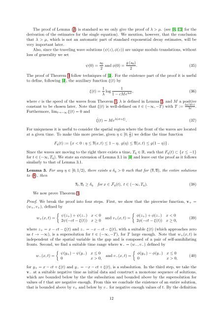
The proof of Lemma (2) is standard so we only give the proof of λ > µ. (see [8, 11] for the
derivation of the estimates for the single equation). We mention, however, that the conclusion
that λ > µ, which is not an automatic part of standard exponential decay estimates, will be
very important later.
Also, since the traveling wave solutions (ψ(z), φ(z)) are unique modulo translations, without
loss of generality we set
ψ(0) = s0
2
g (s0)
and φ(0) = . (35)
2
The proof of Theorem 3 follow techniques of [4]. For the existence part of the proof it is useful
to define, following [4], the auxiliary function ξ(t) by
ξ(t) = 1
λ log
1
, (36)
1 − cMeλct where c is the speed of the waves from Theorem 1, λ is defined in Lemma 2, and M a positive
constant to be chosen later. Note that ξ(t) is well-defined on t ∈ (−∞, −T ) with T := ln(Mc)
λc .
Furthermore, limt→−∞ ξ(t) = 0 and
˙ξ(t) = Me λ(ct+ξ) . (37)
For uniqueness it is useful to consider the spatial region where the front of the waves are located
at a given time. To make this more precise, given η ∈ [0, 1
2 ) we define the time function
Fη(t) := {x < 0 : η ≤ s(x, t) ≤ 1 − η, g(η) ≤ u(x, t) ≤ g(1 − η)} .
Since the waves are moving to the right there exists a time, Tη ∈ R, such that Fη(t) ⊂ {x ≤ −1}
for t ∈ (−∞, Tη). We state an extension of Lemma 3.1 in [4] and leave out the proof as it follows
similarly to that of Lemma 3.1.
Lemma 3. For any η ∈ [0, 1/2), there exists a δη > 0 such that for (s, u), the entire solutions
to (8), then
We now prove Theorem 3.
st, ut ≥ δη for x ∈ Fη(t), t ∈ (−∞, Tη). (38)
Proof. We break the proof into four steps. First, we show that the piecewise function, v+ =
(w+, v+), defined by
ψ(z+) + ψ(z−) x < 0
φ(z+) + φ(z−) x < 0
w+(x, t) =
and v+(x, t) =
(39)
2ψ(−ct − ξ(t)) x ≥ 0
2φ(−ct − ξ(t)) x ≥ 0,
where z+ = x − ct − ξ(t) and z− = −x − ct − ξ(t), with a suitable ξ(t) (which approaches zero
as t → −∞), is a supersolution for t ∈ (−∞, −T ), for T large enough. Note that w+(x, t) is
independent of the spatial variable in the gap and is composed of a pair of self-annihilating
fronts. Second, we find a suitable time range where v− = (w−, v−) defined by
w−(x, t) =
ψ(y+) − ψ(y−) x ≤ 0
0 x > 0,
and v−(x, t) =
φ(y+) − φ(y−) x ≤ 0
0 x > 0,
for y+ = x − ct + ξ(t) and y− = −x − ct + ξ(t), is a subsolution. In the third step, we take the
v− at a suitable negative time as initial data and construct a monotone sequence of solutions,
which are bounded below by the the subsolution and bounded above by the supersolution for
values of t that are negative enough. From this we conclude the existence of an entire solution,
that is bounded above by v+ and below by v− for negative enough values of t. By the definition
12
(40)