Using Hydraulic Head Measurements in Variable ... - Info Ngwa
Using Hydraulic Head Measurements in Variable ... - Info Ngwa
Using Hydraulic Head Measurements in Variable ... - Info Ngwa

You also want an ePaper? Increase the reach of your titles
YUMPU automatically turns print PDFs into web optimized ePapers that Google loves.
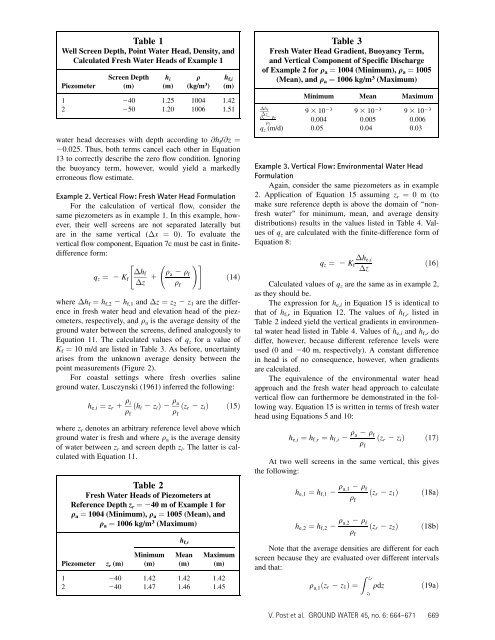
T able 1<br />
W ell Screen D epth, P o<strong>in</strong>t W ater H ead, D ensity, and<br />
C alculated Fresh W ater H eads of E x ample 1<br />
P iezometer<br />
Screen D epth<br />
(m)<br />
water head decreases with depth accord<strong>in</strong>g to @hf/@z ¼<br />
20 .0 25. Thus, both terms cancel each other <strong>in</strong> E quation<br />
13 to correctly describe the zero flow condition. Ignor<strong>in</strong>g<br />
the buoyancy term, however, would yield a markedly<br />
erroneous flow estimate.<br />
E x amp le 2 . Vertical Flow: Fresh Water <strong>Head</strong> Formulation<br />
F or the calculation of vertical flow, consider the<br />
same piezometers as <strong>in</strong> example 1. In this example, however,<br />
their well screens are not separated laterally but<br />
are <strong>in</strong> the same vertical ( x ¼ 0 ) . To evaluate the<br />
vertical flow component, E quation 7 c must be cast <strong>in</strong> f<strong>in</strong>itedifference<br />
form:<br />
qz ¼ 2 Kf<br />
"<br />
hf<br />
z 1<br />
q a 2 q f<br />
q f<br />
! #<br />
ð14Þ<br />
where hf ¼ hf,2 2 hf,1 and z ¼ z2 2 z1 are the difference<br />
<strong>in</strong> fresh water head and elevation head of the piezometers,<br />
respectively, and q a is the average density of the<br />
ground water between the screens, def<strong>in</strong>ed analogously to<br />
E quation 11. The calculated values of qz for a value of<br />
Kf ¼ 10 m/d are listed <strong>in</strong> Table 3. As before, uncerta<strong>in</strong>ty<br />
arises from the unknown average density between the<br />
po<strong>in</strong>t measurements (F igure 2) .<br />
F or coastal sett<strong>in</strong>gs where fresh overlies sal<strong>in</strong>e<br />
ground water, L usczynski (1961) <strong>in</strong>ferred the follow<strong>in</strong>g:<br />
he;i ¼ zr 1 q i<br />
q f<br />
hi<br />
(m)<br />
q<br />
(kg/ m 3 )<br />
hf, i<br />
(m)<br />
1 240 1.25 10 0 4 1.42<br />
2 250 1.20 10 0 6 1.51<br />
ðhi 2 ziÞ 2 qa ðzr 2 ziÞ ð15Þ<br />
qf where zr denotes an arbitrary reference level above which<br />
ground water is fresh and where q a is the average density<br />
of water between z r and screen depth z i. The latter is calculated<br />
with E quation 11.<br />
T able 2<br />
Fresh W ater H eads of P iezometers at<br />
R eference D epth z r ¼ 24 0 m of E x ample 1 for<br />
q a ¼ 10 0 4 (M <strong>in</strong>imum), q a ¼ 10 0 5 (M ean), and<br />
q a ¼ 10 0 6 kg/ m 3 (M ax imum)<br />
P iezometer zr (m)<br />
M <strong>in</strong>imum<br />
(m)<br />
h f, r<br />
M ean<br />
(m)<br />
M ax imum<br />
(m)<br />
1 240 1.42 1.42 1.42<br />
2 240 1.47 1.46 1.45<br />
T able 3<br />
Fresh W ater H ead G radient, B uoyancy T erm,<br />
and V ertical C omponent of Specific D ischarge<br />
of E x ample 2 for qa ¼ 10 0 4 (M <strong>in</strong>imum), qa ¼ 10 0 5<br />
(M ean), and qa ¼ 10 0 6 kg/ m 3 (M ax imum)<br />
M <strong>in</strong>imum M ean M ax imum<br />
hf<br />
z 9 3 10 23 9 3 10 23 9 3 10 23<br />
qa 2 qf q 0 .0 0 4 0 .0 0 5 0 .0 0 6<br />
f<br />
qz (m/d) 0 .0 5 0 .0 4 0 .0 3<br />
E x amp le 3 . Vertical Flow: E nv ironmental Water <strong>Head</strong><br />
Formulation<br />
Aga<strong>in</strong>, consider the same piezometers as <strong>in</strong> example<br />
2. Application of E quation 15 assum<strong>in</strong>g zr ¼ 0 m (to<br />
make sure reference depth is above the doma<strong>in</strong> of ‘ ‘ nonfresh<br />
water’’ for m<strong>in</strong>imum, mean, and average density<br />
distributions) results <strong>in</strong> the values listed <strong>in</strong> Table 4. Values<br />
of q z are calculated with the f<strong>in</strong>ite-difference form of<br />
E quation 8:<br />
qz ¼ 2 Kf<br />
he;i<br />
z<br />
ð16Þ<br />
C alculated values of qz are the same as <strong>in</strong> example 2,<br />
as they should be.<br />
The expression for he,i <strong>in</strong> E quation 15 is identical to<br />
that of h f,r <strong>in</strong> E quation 12. The values of h f,r listed <strong>in</strong><br />
Table 2 <strong>in</strong>deed yield the vertical gradients <strong>in</strong> environmental<br />
water head listed <strong>in</strong> Table 4. Values of he,i and hf,r do<br />
differ, however, because different reference levels were<br />
used (0 and 240 m, respectively) . A constant difference<br />
<strong>in</strong> head is of no consequence, however, when gradients<br />
are calculated.<br />
The equivalence of the environmental water head<br />
approach and the fresh water head approach to calculate<br />
vertical flow can furthermore be demonstrated <strong>in</strong> the follow<strong>in</strong>g<br />
way. E quation 15 is written <strong>in</strong> terms of fresh water<br />
head us<strong>in</strong>g E quations 5 and 10 :<br />
he;i ¼ hf;r ¼ hf;i 2 q a 2 q f<br />
q f<br />
ðzr 2 ziÞ ð17 Þ<br />
At two well screens <strong>in</strong> the same vertical, this gives<br />
the follow<strong>in</strong>g:<br />
he;1 ¼ hf;1 2 q a;1 2 q f<br />
q f<br />
he;2 ¼ hf;2 2 q a;2 2 q f<br />
q f<br />
ðzr 2 z1Þ ð18aÞ<br />
ðzr 2 z2Þ ð18bÞ<br />
Note that the average densities are different for each<br />
screen because they are evaluated over different <strong>in</strong>tervals<br />
and that:<br />
q a;1ðzr 2 z1Þ ¼<br />
Z zr<br />
z1<br />
qdz ð19aÞ<br />
V. P ost et al. GROUND WATER 45, n o. 6: 664–671 669