Basics of Electrochemical Impedance Spectroscopy - Gamry ...

Figure 1. Sinusoidal Current Response in a Linear
System
The excitation signal, expressed as a function of time,
has the form
E = E sin( t)
t 0 ω (2)
where E t is the potential at time t, E 0 is the amplitude
of the signal, and ω is the radial frequency. The
relationship between radial frequency ω (expressed in
radians/second) and frequency f (expressed in hertz) is:
ω = 2π f (3)
In a linear system, the response signal, I t , is shifted in
phase (φ) and has a different amplitude, I 0 .
I = I sin ( t + )
t 0 ω φ (4)
An expression analogous to Ohm's Law allows us to
calculate the impedance of the system as:
Z
Et
E0 sin( ω t)
= =
= Z
I I sin( ω t + φ)
t
0
0
sin( ω t)
sin( ω t + φ )
(5)
The impedance is therefore expressed in terms of a
magnitude, Z o , and a phase shift, φ.
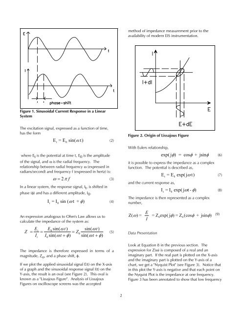
If we plot the applied sinusoidal signal E(t) on the X-axis
of a graph and the sinusoidal response signal I(t) on the
Y-axis, the result is an oval (see Figure 2). This oval is
known as a "Lissajous Figure". Analysis of Lissajous
Figures on oscilloscope screens was the accepted
2
method of impedance measurement prior to the
availability of modern EIS instrumentation.
Figure 2. Origin of Lissajous Figure
With Eulers relationship,
exp( j φ) = cos φ + jsinφ
(6)
it is possible to express the impedance as a complex
function. The potential is described as,
and the current response as,
E = E exp( j t)
t 0 ω (7)
I = I exp( j t - )
t 0 ω φ (8)
The impedance is then represented as a complex
number,
E
Z( ω) = = Z0exp( j φ) = Z 0 (cos φ + jsinφ)
I
(9)
Data Presentation
Look at Equation 8 in the previous section. The
expression for Z(ω) is composed of a real and an
imaginary part. If the real part is plotted on the X-axis
and the imaginary part is plotted on the Y-axis of a
chart, we get a "Nyquist Plot" (see Figure 3). Notice that
in this plot the Y-axis is negative and that each point on
the Nyquist Plot is the impedance at one frequency.
Figure 3 has been annotated to show that low frequency