Turbulent flows generated/designed in multiscale/fractal ... - Ercoftac

first session | Fundamentals
Fundamentals | first sessioN
monday 28 MARCH 2011 | 9.50-10.25
MONDAY 28 MARCH 2011 | 9.15-9.50
Freeing turbulence
from the tyranny of
the past
W.K. George
Department of Aeronautics, Imperial College London, UK
There have been numerous studies over the past few decades about how
scientists do research on difficult and intractable problems, both how we function
as individuals and collectively. While we would like to think that as individuals we
are purely objective, all evidence suggests that we are not, and our judgements are
strongly influenced by intuition and past prejudices. In groups we tend to cluster
around ‘group-think’, substituting consensus for critical analysis. Moreover there is
a ‘herd’ instinct, meaning there is a tendency to flock to a new idea, often without a
good reason for doing so.
Of course none of this behaviour has ever happened in turbulence. Nonetheless,
by examining the problems those in other fields have had, we can learn how to
guard against them in the future. Therefore the first part of this presentation will
focus on the phenomena of how we function as turbulence researchers. And the
second will try to identify potential problem areas where if we are not careful ideas
we have long assumed to be true might be adopted as religious principles, even if
they are false or only partially true.
Also in this talk we will try to distinguish between the mathematics of turbulence
and the physics of turbulence. In mathematics, equations are precisely determined,
and the laws of mathematics which must be applied to find solutions are welldefined
Physicists, on the other hand, build mathematical models of the universe
as we find it. Once we have built the model and defined the boundary conditions,
however, there is nothing that is arbitrary: the laws of mathematics take over. The
problem in turbulence (and other fields as well) is that often the consequences
of the mathematics for our solutions are not consistent with what we observe in
nature. So is the problem with our model, or is it with the boundary conditions
we have assumed to be true? Since often we have had to assume these to be
applied at infinity, we cannot be sure. Nonetheless, there are usually some criteria
for evaluation we can agree upon. For example if our model is the Navier-Stokes
equations, it should not generally be our first assumption that they are wrong,
especially for the constant density flow of a Newtonian fluid. Nor should we throw
away so quickly a theory developed for an infinite domain if our experiment is
performed in a box. In fact it will probably be more productive to examine what
the consequences are of the finite domain or our attempts to realize the solution in
nature. Numerous examples will be used to illustrate these points [1,2,3,4,5].
Beyond mean flow scaling
laws - how to obtain higher
order moment scaling from
new statistical symmetries
1 st UK-JAPAN BILATERAL WORKSHOP, IC LONDON, UNITED KINGDOM, 28./29.3.2011
BEYOND MEAN FLOW SCALING LAWS - HOW TO OBTAIN HIGHER ORDER MOMENT
M. Oberlack 1,2,3 , A. Rosteck 1 UK-JAPAN 3 BILATERAL SCALING FROM WORKSHOP, NEW STATISTICAL IC LONDON, SYMMETRIES
UNITED KINGDOM, 28./29.3.2011
1 1
Chair of Fluid st UK-JAPAN BILATERAL WORKSHOP, IC LONDON, UNITED KINGDOM, 28./29.3.2011
Dynamics, BEYOND MEAN Technische FLOW SCALING Universität Darmstadt, GERMANY
Martin Oberlack LAWS 1,2,3 - HOW & Andreas TO OBTAIN Rosteck 1 HIGHER ORDER MOMENT
2
Center of BEYOND Smart MEAN Interfaces, 1 Chair FLOW of Fluid SCALING TU Dynamics SCALING
Darmstadt, LAWS , Technische FROM - HOW NEW Universität Germany
TO STATISTICAL OBTAIN Darmstadt, HIGHER SYMMETRIES
64289 Darmstadt, ORDER MOMENT Germany,
1 st UK-JAPAN
3
GS Computational Engineering, 2 BILATERAL WORKSHOP, IC LONDON, UNITED
SCALING CenterFROM of Smart NEW Interfaces, STATISTICAL TU Darmstadt, SYMMETRIES
KINGDOM, 28./29.3.2011
64287 Darmstadt, Germany
TU Darmstadt, Germany
3 GS Computational
Martin
Engineering,
Oberlack
TU 1,2,3 Darmstadt,
& Andreas
64293
Rosteck
Darmstadt, 1
BEYOND 1 MEAN FLOW SCALING LAWS - HOW TO OBTAIN HIGHER ORDER GermanyMOMENT
Chair of Fluid Dynamics , Technische Universität Darmstadt, 64289 Darmstadt, Germany,
We investigate the symmetry We investigate and the symmetry 2 Martin SCALING Oberlack FROM
invariance Center and of Smart invariance structure 1,2,3 NEW & Andreas STATISTICAL RosteckSYMMETRIES
Interfaces, structure TUof Darmstadt, of the infinite 1
1 64287 set of set Darmstadt, multi-point of multi-point Germany correlation correlation (MPC) equations
for the fluctuations velocity 3 , Technische Universität Darmstadt, 64289 Darmstadt, Germany,
2 GS and Computational pressure u(x, t) fluctuations and
(MPC) equations for
Chair of Fluid Dynamics
the velocity and pressure
Engineering,
p(x, u(x, t) t) TUand Darmstadt, p(x, t) 64293 Darmstadt, Germany
Center of Smart Interfaces, Martin TUOberlack Darmstadt, 1,2,3 & 64287 Andreas Darmstadt, Rosteck 1 Germany
3 GS 1 Computational Chair of Fluid Dynamics Engineering,
, Technische TU Darmstadt, Universität64293 Darmstadt, Darmstadt, 64289 Darmstadt, Germany Germany,
We investigate the
S i{n+1} = ∂R symmetry and
i {n+1}
n invariance structure
+ Ū k(l) (x
∂t
(l) ) ∂R of the infinite
i {n+1}
− ν ∂2 R i{n+1}
set of multi-point correlation (MPC) equations
for the velocity 2 Center of Smart Interfaces, TU Darmstadt, 64287 Darmstadt, + R Germany
3 and pressure fluctuations u(x,
∂Ūi (l)
∂x
t) and p(x,
k(l) ∂x
t)
k(l) ∂x
i{n+1} [i (l) →k (l) ]
GS Computational k(l) ∂x k(l)
l=1
Engineering, TU Darmstadt, 64293 Darmstadt, Germany
We investigate the symmetry and invariance structure
∂u i(l) u k(l) (x (l) )
− R i{n} [i (l) →0]
+ ∂P i {n} [l]
+ ∂R (1)
i {n+2} [i (n+1) →k (l) ][x (n+1) → x (l) ]
S i{n+1} = ∂R of the infinite set of multi-point correlation (MPC) equations
for the + Ū k(l) (x ,
i {n+1}
n
∂t
(l) ) ∂R i {n+1}
− ν ∂2 R i{n+1}
∂Ūi (l)
We
velocity
investigate
and pressure
the symmetry
fluctuations
and invariance
u(x, t)
structure
and p(x,
of
t)
the infinite set of multi-point + R
∂x k(l)
∂x ∂x k(l) i(l)
∂x k(l) ∂x
i{n+1} correlation [i
∂x
(l) →k (l) ] (MPC) equations
for the velocity and pressurel=1
fluctuations u(x, t) and p(x, t)
k(l) k(l)
∂x k(l)
∂u i(l) u k(l) (x (l) )
where n =1...∞. − RIn i{n} (1)[i the (l) →0] MPC tensor is defined + ∂P i {n} [l]
as R i{n+1} + ∂R (1)
S i {n+2} [i (n+1) →k (l) ][x (n+1) → x (l) ]
= u i(0) (x (0) ) · ...· u i(n) (x (n) ) , and with , the
four variations S i{n+1} of = ∂R
i{n+1} = ∂R
i {n+1}
n
+ Ū k(l) (x
∂t i {n+1}
n (l) ) ∂R i {n+1}
it we have + a complete Ū k(l)
∂x
statistical k(l) (x ∂x
description i(l) ∂x
of turbulence. k(l)
∂t
(l) ) ∂R − ν ∂2 R i{n+1}
∂Ūi (l)
+ R
∂x i {n+1}
− ν ∂2 k(l) ∂x k(l) ∂x R i{n+1} [i i{n+1}
(l) →k (l) ]
k(l) ∂x
+ R k(l)
∂Ūi (l)
l=1
∂x k(l) ∂x k(l) ∂x
i{n+1} [i (l) →k (l) ]
k(l) ∂x k(l)
Equation (1) admits∂u l=1
all i(l) symmetries u k(l) (x (l) of ) the Navier-Stokes equations where they originally emerged from at the
where n =1...∞. In (1) the
first place. Nevertheless equation ∂uMPC i(l) (1) upossesses k(l)
tensor (x (l) ) is defined as R
additional symmetries i{n+1} = u
(see i(0) (x
Oberlack, (0) ) · ...· u
Rosteck i(n) (x
2010 (n) ) , and with the
& Rosteck
four variations− of Rit Oberlack 2011)
i{n} we[i (l) have →0] a complete statistical + ∂P i {n} [l]
description + ∂R (1)
− R i{n} [i (l) →0]
+ ∂P i {n} [l]
+ ∂R (1)
i {n+2} [i (n+1) →k (l) ][x (n+1) → x (l) ]
i {n+2} [i (n+1) →k (l) ][x (n+1) → x (l) ],
∂x k(l) ∂x i(l) of turbulence. ∂x k(l)
,
∂x k(l) ∂x i(l) ∂x k(l)
Equation (1) admits all symmetries of the Navier-Stokes equations
G sh : ˜x = x, ˜r i(l) = r i(l) , ˜Ū i = e asŪ i, ˜R ij (x, y) =e where they originally emerged as (1 − e as )Ūi(x)Ūj(y) − R ij (x, y) from at the
where n =1...∞. first place. In (1) Nevertheless MPC equation tensor is(1) defined possesses as Radditional symmetries (see Oberlack, Rosteck 2010 , ··· & Rosteck
where n =1...∞. In (1) the MPC tensor is defined i{n+1} = u
as R i(0) (x
i{n+1} = u (0) ) · ...· u
i(0) (x
Oberlack 2011)
(0) ) · ...· i(n) (x
u (n) ) , and with the
i(n) (x (n) ) , and with the
four variations
four
of
variations
it we have
G L(a) : ˜x of= it
a complete
x, we˜r have
i(l) = arcomplete statistical
i(l) , ˜Ū i = statistical
description Ūi + L (i) , description
of turbulence.
of turbulence.
Equation (1) Equation admits all (2)
G
(1) symmetries admits
sh : ˜R ij
˜x (x, =
all
x,
symmetries of the Navier-Stokes
y) ˜r =R i(l) = ij (x, r i(l) y) ,
of
− ˜Ū the i L =
Navier-Stokes
e (i) Ū asŪ equations
j (y) i, − ˜R ij L (x, (j) Ūy) equations where
i (x) =e − as L (1
where they originally
(i) L − e (j) , as they
··· )Ūi(x)Ūj(y)
originally emerged
−
emerged from
R ij (x, y)
from at
, ···
at the the
first place. Nevertheless first place. Nevertheless equation (1) equation possesses (1)
G L(ab)
G : ˜x = x, ˜r i(l) = r i(l) , ˜Ū L(a) : ˜x = x, ˜r i = Ūi, ˜R i(l) = r i(l) , ˜Ū
possesses additional additional symmetries symmetries (see Oberlack, (see Oberlack, Rosteck Rosteck 2010 2010 & & Rosteck
Oberlack 2011) Oberlack 2011)
i = + ij
L (x, (i) , y) =R ij (x, y)+L (ij) , ···
(2)
˜R ij (x, y) =R ij (x, y) − L (i) Ū j (y) − L (j) Ū i (x) − L (i) L (j) , ···
G The latter G sh are : ˜x purely x, statistical ˜r i(l) = r i(l) properties , ˜Ū i of the equations (1), while G sh can be identified as a statistical scaling
group G(SSG) L(ab) and : ˜x G= L(a)
x, ˜r , i(l) G L(ab)
= r i(l) as, statistical ˜Ū
= e asŪ i, ˜R
i = Ūi, translation ˜R
ij (x, y) =e as (1 − e as − R ij (x, y) sh : ˜x = x, ˜r i(l) = r i(l) , ˜Ū i = e asŪ i, ˜R ij (x, y) =e as − e as )Ūi(x)Ūj(y) − R ij (x, y) , ··· , ···
ij (x, y) =R groups ij (x, (STG). y)+L (ij) , ···
G G
Assuming L(a) : ˜x x, ˜r i(l) r i(l) , ˜Ū i =
a plane parallel turbulent shear Ūi + L
flow, (i) ,
L(a) : ˜x = x, ˜r i(l) = r i(l) , ˜Ū i = the infinite set of equations (1) and the corresponding symmetries
provide the
The latter are purely statistical Ūi + L (i) ,
properties of the equations (1), while G ˜R ij invariant (x, y) =Rsurface ij (x, y) condition − L sh can be identified as a statistical scaling
(i) Ū j (y) − L (j) Ū i (x) − L (i) L (j) , ···
(2)
(2)
˜R group ij (x,(SSG) y) =Rand ij (x, G L(a)
y) , −G L L(ab) (i) Ūas statistical translation groups (STG).
Assuming
G L(ab) :
a
˜x
plane x,
parallel
˜r i(l) = r
dx 2 turbulent i(l) , ˜Ū
j (y) − L (j) Ū i (x) − L (i) L (j) , ···
i
= dr =
shear Ūi,
(k) flow, ˜R ij (x,
the
y)
infinite
=R ij (x,
dŪ1 set
y)+L
of equations
=
= dR (ij) , ···
G (11)(x, (1) y) and the corresponding symmetries
provide the invariant
L(ab) : ˜x = x, ˜r i(l) = r i(l) , ˜Ū i = = ··· (3)
k 1 x 2
surface Ūi, ˜R ij (x, y) =R ij (x, y)+L (ij) , ···
+ k x kcondition
The latter are purely statistical properties 1 r (k) of the (kequations 1 − k 2 + k(1), a )Ū1 while + l 1 G sh can I(x, bey)
identified as a statistical scaling
The latter aregroup purely (SSG) statistical and G
with the group parameters L(a)
properties , G
k L(ab)
of
dx asthe statistical equations
1 , k 2 2 , k
= x , k dr translation (1), while groups G sh (STG). can be
a ,(k)
l 1 and
=
l 11 descending dŪ1 from the
= dR identified
groups (11)(x,
(2) y) as a statistical scaling
and
= ···
the classical symmetry
group (SSG) Assuming and G (3)
groups here L(a) a , plane G
written L(ab) parallel as statistical
in infinitesimal k turbulent 1 x 2 + k shear translation
x forms. k 1 r flow,
(k) (k
the groups
1 −
infinite(STG).
k 2 + k
set of a )Ū1 +
equations
l 1 I(x, (1) and y) the corresponding symmetries
provide parallel theturbulent invariant surface shear flow, condition the infinite set of equations (1) and the corresponding symme-
Assuming a plane
tries provide the with invariant the group surface parameters condition k 1 , k 2 , k x , k a , l 1 and l 11 descending The abbreviation from the groups I(x, y) (2) isandefined the classical I(x, symmetry y) =
groups here written in infinitesimal dx 2
= dr forms. (k)
dŪ1
=
[2k 1 − 2k= 2 + dR k a
(11)(x, y)
]R (11) (x, = y)+l ··· 11 − k a Ū i (x)Ūj(y) (3) −
dx k 1 x 2 + k x k 1 r (k) (k 1 − k 2 + k a l)Ū1 1 (Ūi(x)+Ūj(y)) + l 1 I(x, and y)
2
the indices in brackets denote
= dr (k)
dŪ1
=
no
The = dR (11)(x, y)
summation
abbreviation
but instead = I(x, ··· y)
each
is defined
component
as I(x,
is (3) to
y)
be
=
with the group k 1 xparameters 2 + k x k 11 r , (k) k 2 , k x
(k , k 1a −, l 1
k 2 and + lk 11 a )Ū1 descending + l 1
taken
[2k 1
from
separately.
−
I(x,
2kthe 2 +
y) groups k a ]R (11)
(2)(x, and y)+l the classical 11 − k a Ū i
symmetry (x)Ūj(y) −
groups here written in infinitesimal forms.
From
l 1 (Ūi(x)+Ūj(y))
(3) we may derive
and
various
the indices
new
in
scaling
brackets
laws
denote
with the group parameters k 1 , k 2 , k x , k a , l 1 and l 11 descending from the groups (2) and the classical symmetryfor
the
no
MPC
summation
tensor. Presently,
but instead
we
each
invoke
component
symmetries
is to
in
be
groups here written in infinitesimal forms.
The abbreviation I(x, y) is defined as I(x, y) =
the
taken
range
separately.
[2k of the validity of the logarithmic law of the
wall
From 1 − 2k
i.e.
(3) 2 + k
k 1 −
we a ]R
k
may (11) (x, y)+l
2 + k
derive
a =0and
various 11 − k
compute
new a Ū
scaling i (x)Ūj(y) −
the Reynolds
laws for
The abbreviation l 1 (Ūi(x)+Ūj(y)) I(x, y) andisthedefined indices in asbrackets I(x, y) denote =
stresses
the MPC
in
tensor.
the range
Presently,
or the logarithmic
we invoke symmetries
law of the
in
[2k 1 −no 2ksummation - but -instead each- component - is to be
wall.
the 2 + range k a ]R
The parameters
of (11) the(x, validity y)+l
of the
of 11
new
the − k
equations
logarithmic a Ū i (x)Ūj(y)
describing
law−of the
l 1 (Ūi(x)+Ūj(y)) taken separately.
the
wall
Reynolds
i.e. k 1 −and stresses
k 2
the + kindices have a =0and in
been determined
compute bracketsthe denote
from
Reynolds
From (3) we may derive various new scaling laws for the
no summation
DNS-data
stressesbut in
of
the instead
a boundary
rangeeach or
layer
the component logarithmicis flow at Re
law to be
Θ = 2003
of the
separately. the MPC tensor. Presently, we invoke symmetries in
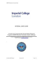
Figure 1. Comparison of the DNS data (dotted lines) with taken separately.
by
wall.
Hoyas
The
and
parameters
Jimenez
of
(2006).
the new
In
equations
figure 1
describing
the range of the validity of the logarithmic lawone of the can
the scaling laws resulting from the new symmetries (solid From (3) see
the we that
Reynolds may thisderive provides
stresses various have
excellent new beenscaling determined
matchlaws in the
from for log
the
wall i.e. k
lines)
region.
DNS-data 1 − k
of 2 + k
a boundary a =0and compute the Reynolds
the MPC layer flow at Re Θ = 2003
stresses tensor. in the Presently, range or wethe invoke logarithmic symmetries law ofinthe
Figure 1. Comparison of the DNS data (dotted lines) the with rangeby Hoyas and Jimenez (2006). In figure 1 one can
wall. ofThe theparameters validity of of the thelogarithmic new equations lawdescribing
of the
the scaling laws resulting from the new symmetries (solid see that this provides an excellent match in the log
wall i.e. the k 1 Reynolds − k 2 + kstresses a =0and havecompute been determined the Reynolds from the
lines)
region.
stressesDNS-data in the range of a boundary or the logarithmic layer flow at law Re Θ of = the 2003
Figure 1. Comparison of the DNS data (dotted lines) with wall. The by Hoyas parameters and Jimenez of the new (2006). equations In figure describing 1 one can
the scaling laws resulting from the new symmetries (solid the Reynolds see thatstresses this provides have been an excellent determined matchfrom in the the log
lines)
DNS-data region. of a boundary layer flow at Re Θ = 2003
Figure 1. Comparison of the DNS data (dotted lines) with by Hoyas and Jimenez (2006). In figure 1 one can
the scaling laws resulting from the new symmetries (solid see that this provides an excellent match in the log
lines)
region.
where n=1...∞. In (1) the MPC tensor is defined as
have a complete statistical description of turbulence.
and with the four variations of it we
Equation (1) admits all symmetries of the Navier-Stokes equations where they originally emerged from in the first place.
Nevertheless equation (1) possesses additional symmetries (see [6,7])
The latter are purely statistical properties of the equations (1), while G sh
can be identified as a statistical scaling group
(SSG) and G L(a)
, G L(ab)
as statistical translation groups (STG).
Assuming a plane parallel turbulent shear flow, the infinite set of equations (1) and the corresponding symmetries provide
the invariant surface condition
with the group parameters k 1
, k 2
, k x
, k a
, l 1
and l 11
descending from the groups (2) and the classical symmetry groups here
written in infinitesimal forms.
The abbreviation I(x, y) is defined as: I(x, y) = [2k 1
- 2k 2
+ k a
]R (11)
(x,y) + l 11
- k a
U i
(x)U j
(y) - l 1
(U i
(x) + U j
(y)) and the indices in brackets
denote no summation but instead each component is to be taken
From (3) we may derive various new scaling laws for the MPC
tensor. Presently, we invoke symmetries in the range of the validity
of the logarithmic law of the wall i.e. k 1
− k 2
+ k a
= 0 and compute
the Reynolds stresses in the range or the logarithmic law
of the wall. The parameters of the new equations describing the
Reynolds stresses have been determined from the DNS-data of
a boundary layer flow at Re τ
= 2003 by Hoyas and Jimenez [8].
In figure 1, one can see that this provides an excellent match in
the log region.
4 turbulent flows generated/designed in multiscale/fractal ways: fundamentals and applications
turbulent flows generated/designed in multiscale/fractal ways: fundamentals and applications 5