Download - ePub WU

More documents

Recommendations

Info

652 JOURNAL OF CONSUMER RESEARCH et al. 1994, 1996; Goldenberg et al. 2008; Myers and Robertson 1972; Venkatraman 1989). Knowledgeable and influential consumers have also been conceptualized and operational ized as "market mavens" (Feick and Price 1987). We incorporated all tbree characteristics of opinion leadership into a concise 3-indicator scale for children. A Cronbach's alpha of .79 showed that the internal consistency of the three indicators was sufficiently high. Therefore, the indicators were combined into a single scale for opinion leadership. Confirmatory factor analysis revealed a good overall fit (GFI = .93; IFI = .93; CFI = .92). In addition, all three indicators loaded positively and statistically significantly on opinion leadership (/J< .01), thus pointing to a satisfactory level of convergent validity. Self-reported measures are often criticized in the literature on adults, mainly with the argument that some people are unable to report their performance accurately due to poor introspection (Locke, Latham, and Erez 1988). However, there are also many studies that use self-reported measures and achieve high levels of accuracy (Cooper 1981). In addition, there are concepts that can hardly be measured objectively, for example, "individual creativity" (Leenders. van Engelen, and Kratzer 2007). This is also tbe case witb tbe concepts of lead usemess and opinion leadership. Throughout tbe literature, the measurement of lead usemess and opinion leadership is widely based on self-reported values. We tbus adapted our measurements to existing operationaiizations and used self-reported values. Moreover, there is evidence that self-ratings correlate highly with more "objective" measures in cases wbere anonymity is assured. In particular, Heneman (1974) found tbat self-reported measures were less restricted in range and leniency than tbe purportedly more objective ratings. Accordingly, we also promi.sed anonymity in our study. In addition, Corey (1971) and Tittle and Hill ( 1967) argue that the error arising from self-reporting techniques is minor. In fact, our results enable a clear classification along tbe dimensions of lead userness and opinion leadership. As shown below, we also find roughly the same association between lead userness and opinion leadership (table I ; r = 0.34) as that reported in prior studies on adults (Morrison et al. 2000; Schreier et ai. 2007). Control Variable.^, There are many other factors that have been shown to influence (or that may influence) behavioral effects witbin social networks. While it is not possible to include all other variables in tbis study, we chose to include two variables that have demonstrated the most prominent effect on tbe social networks of children. First. we included gender because males and females express and satisfy their needs and feelings differently (Del Vecchio 2002). In addition, Kalmijn (2003) reports that gender influences social networks because females are likely to bave more frequent contact witb friends than males do. This variable is included as a dummy, where male = 0 and female = I. Second, we included age because children of different ages have differing likes and dislikes and because children's thoughts, expectations, and feelings change as tbey grow older (John and Lakshmi-Ratan 1992). In addition, research shows that social networks are not stable over time. Stages in the course of an actor's life will also influence his or her social networks (Kalmijn 2003). Analytical Techniques In order to test hypotheses 1 and 2, we used hierarchical linear modeling (HLM). This method has its origins in research performed at schools, which are also the setting of this study, but many organizational pbenomena (e.g., the behavior of individuals within teams) also occur as hierarchically ordered systems, with variables of interest residing at different levels of analysis (Hoffman, Griffin, and Gavin 2000). The HLM methodology is particularly well suited for analyzing hierarchically nested data structures where micro-level observations (i.e., individuals) are nested within macro-level observations (i.e., scbool classes/teams; Bryk and Raudenbush 1992). Hierarcbical linear modeling explicitly recognizes that individuals within school classes/ teams may be more similar to eacb other than to individuals in other school classes/teams and therefore may not provide independent observations (Hoffman et al. 2000). In order to test wbetber the observations are indeed nested in scbool classes, we calculated tbe intraclass correlation coefficients (ICCs) for lead userness and opinion leadersbip. The results show a moderate ICC for lead usemess (.64) and opinion TABLE 1 DESCRIPTIVE STATISTICS AND CORRELATION COEFFICIENTS Variable Mean SD 1. Lead user 2. Opinion leader 3. Gender 4. Age 5. Degree centrality 6. Closeness centrality 7. Betweenness centrality 3.12 2.93 .53 8.76 39.17 25.60 16.30 .45 .88 .51 1.31 10.76 8.33 19.75 .34" 17" 09- .25" .12- -.11" .09- .59" .02 .21" .23" .32" -.09- .11- .37" .61 .22 .06 .17 .41 .39 NOTE.—W= 519. •p
NETWORK SIDE OF LEADING EDGE CONSUMERS 653 leadership (.72; Shrout and Fleiss 1979). These moderate ICC scores justify tbe use of hierarchical linear models. For nested data, HLM analysis is not only more accurate but is in fact preferred to other approaches (e.g., ordinary least squares estimation) that do not estimate variance separately at the individual and group levels (Sarin and McDermott 2003), In HLM. the lower-level analysis is also referred to as level 1, while the higher-level analysis is referred to as level 2. In our analyses, level 1 refers to the children and level 2 refers to the 23 school classes. At level 1, we include two dependent variables (lead usemess and opinion leadership), three independent variables (individual network coefficients: betweenness. degree, and closeness cenirality), and two controls (age and gender). The level 1 variables in an HLM model will allow us to determine a simple level 2 variation. In other words, we can determine whether or not the results vary among the 23 school clas.ses. However, the individual network measures depend on the total number of ties within each of the 23 school classes. 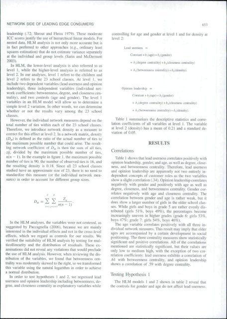Therefore, we introduce network den.sity as a measure to correct for this effect at level 2. In a network matrix, density (D^) is defined as the ratio of the actual number of ties to tbe maximum possible number that could arise. The resulting network coefficient of D^ is then the sum of all ties. zij, divided by the maximum possible number of ties, n(n - I ). In the example in tigure I, the maximum possible number of ties is 90. the number of observed ties is 16, and tbe resulting density is 0.18. Since all 23 scboo! classes studied have an approximate size of 23. there is no need to standardize this measure (or the individual network measures) in order to account for different group sizes. in tbe HLM analyses, tbe variables were not centered, as suggested by Paccagnella (2006), becau.se we are mainly interested in tbe individual effects and not In the cross-level effects, which we regard as controls for our results. We verified the suitability of HLM analysis by testing for multicollinearity and the distribution of residuals. These examinations did not reveal any violations that would preclude the use of HLM analysis. However, when reviewing the distribution of the variables, we found that betweenness centrality was moderately skewed to the right, so we transformed this variable using the natural logarithm in order to achieve a normal distribution. In order to test hypotheses 1 and 2, we regressed lead usemess and opinion leadership including betweenness, degree, and closeness centrality as explanatory variables while controlling for age and gender at level I and for density at level 2: Lead userncss = Constant + h, (age) + &, (gender) + />,(degree centrality)+ è^(closeness centrality) + È,(betweenness cenirality)+&o(density). Opinion le^lership = Constant+è|(age)+i>j(gender) + fej(degree cemraUty)+fcj(closeness centrality) + /»s(betweenness centrality)+ft^(density). Table I summarizes tbe descriptive statistics and correlation coefficients of all variables at level I. The variable at level 2 (density) has a mean of 0.21 and a standard deviation of 0.05. Correlations RESULTS Table 1 shows tbat lead userness correlates positively with opinion leadership, gender, and age. as well as degree, closeness, and betweenness centrality. Therefore, lead userness and opinion leadership are apparently not two entirely independent concepts of customer roles as the two variables show a slight correlation (.34). Opinion leadership correlates negatively with gender and positively with age as well as degree, closeness, and betweenness centrality. Gender correlates negatively witb age and closeness centrality. The correlation between gender and age is rather weak, but it does show a larger number of girls in the older school classes. While girls and boys in grade 5 are rather evenly distributed (girls 51%. boys 49%), tbe percentages become increasingly uneven in higher grades (grade 6: girls 53%, boys 47%: grade 7: girls 54%, boys 46%), Tbe age variable correlates positively witb all three individual network measures. This result may imply that older ages are accompanied by a cenain development in social positioning. The three centrality measures show statistically significant and positive correlations. All of the correlations mentioned are statistically significant, but their values are only low to medium high, with the exception of two correlation coefficients: lead userness exhibits a correlation of .61 with betweenness centrality, and opinion leadership shows a correlation of .59 with degree centrality. Testing Hypothesis 1 The HLM models I and 2 shown in table 2 reveal that the controls for gender and age do not affect lead usemess.
Page 1 and 2: ePub WU Institutional Repository Ja
Page 3 and 4: NETWORK SIDE OF LEADING EDGE CONSUM
Page 7: NETWORK SIDE OF LEADING EDGE CONSUM

Download - ePub WU

You also want an ePaper? Increase the reach of your titles

Delete template?

Save as template?