Diversity, Abundance and Species Composition of Water ... - Idosi.org

Acad. J. Entomol., 4 (2): 64-71, 2011
Table 3: Alpha diversity indices for different sites at Kolkas region of Melghat Tiger Reserve
Index Site I Site II Site III Site IV Site V
Fisher -diversity 8.27 7.957 7.478 3.947 5.965
Shannon H' 3.295 3.146 3.001 2.588 2.892
Simpsons (D) 0.071 0.079 0.11 0.166 0.119
Hills No (H0) 11 10 10 8 9
Shannon J 0.952 0.947 0.903 0.863 0.912
8
Abundance Plot
15
Rarefaction Plot
6
10
Abundance
4
Site I
2
Site II
Site III
Site IV
Site V
0
1 10 100
Rank
Fig. 5: Species rank abundance plot for five different sites
ES(n)
5
n
Site I
Site II
Site III
Site IV
Site V
0
0 5 10 15 20 25
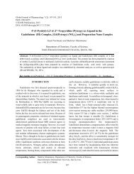
Fig. 6: Sample based rarefraction curve for different sites
site III (3.00), site V (2.89) and lastly the site IV (2.58). The
Simpson and Shannon J (evenness) indices also revealed
almost the same order of diversity of sites (Table 3).
Species were ranked according to their abundance.
Common species are displayed on the left and the rare
species are on the right (Fig. 5). Abundance ranking
showed that Site IV had less number of rare species
(i.e. abundance value 2) and more number of common
species (i.e. abundance value 7) as compared to other
sites. Site I and II were comparable to each other and so
was the case with site III and V.
Sample Based Rarefraction Curve for Five Different
Transects: Rarefraction curve is shown in Fig. 6. Expected
number of species [ES(n)] has been plotted against
number of individuals (n). This plot provides a measure of
species diversity. Steeper curve indicated more diverse
communities. A steeper curve was observed for site I
because of its high species diversity. Site II was almost
equally rich followed by site III. Sites V and IV were low
in diversity.
Comparison of Species Turnover among Transects:
To visualize difference in species composition between
the different sites (habitats), a complete linkage of Jaccard
(Jaccard similarity matrix- presence/absence)
Fig. 7: Dendrogram comparing different sites by their
water beetle species assemblage
similarity and Bray Curtis coefficient matrix was carried
out. The dendrogram clustering of the species grouping
and habitats grouping was drawn. Jaccard similarity
indices were calculated based on presence and absence
of particular taxa at different study sites of Kolkas region,
whereas Bray Curtis coefficient clustering was calculated
based on the similarity richness and abundance of water
beetle taxa.
The Jaccard similarity matrix showed very close
similarity between the site V and site III which form a
single cluster and site I and site II formed another cluster.
68