Do the Hodrick-Prescott and Baxter-King Filters Provide a ... - UQAM

DO THE HODRICK-PRESCOTT AND BAXTER-KING FILTERS PROVIDE A GOOD
APPROXIMATION OF BUSINESS CYCLES? 19
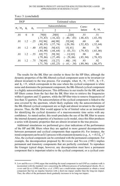
TABLE 3: (concluded)
DGP
σε
/ ση
1
φ φ2
.01 0 0 .79[0]
(.75,.83)
.01 1.2 – .25 .91[.96]
(.88,.93)
.01 1.2 – .40 .87[.86]
(.84,.90)
.01 1.2 – .55 .83[.77]
(.79,.86)
.01 1.2 – .75 .74[.69]
(.71,.78)
Autocorrelations
Estimated values
1 2 3
.29[0]
(.16,.42)
.66[.90]
(.57,.74)
.54[.63]
(.44,.64)
.39[.38]
(.27,.49)
.13[.27]
(.03,.23)
– .22[0]
(– .40,– .03)
.35[.84]
(.20,.50)
15[.41]
(– .03,.31)
– .11[.03]
(– .29,.06)
– .48[– .19]
(– .61,– .34)
Correlation
σˆ / σ
.55
(.48,.63)
.68
(.52,.82)
.86
(.79,.92)
.90
(.85,.94)
.93
(.89,.96)
c
c
.51
(.43,.58)
.48
(.32,.64)
.76
(.65,.86)
.86
(.78,.92)
.92
(.86,.97)
The results for the BK filter are similar to those for the HP filter, although the
dynamic properties of the BK-filtered cyclical component seem to be invariant (or
almost invariant) to the true process. For example, when σε
/ σ u = 0.01, φ 1 = 0 ,
and φ 2 = 0 , which corresponds to the case where the cyclical component is white
noise and dominates the permanent component, the BK-filtered cyclical component
is a highly autocorrelated process. This difference in our results for the BK and the
HP filters comes from the fact that the BK filter tries to retrieve the frequencies
within 6 quarters and 32 quarters, while the HP filter tries to remove frequencies of
less than 32 quarters. The autocorrelation of the cyclical component is linked to the
area covered by the spectrum, which likely explains why the autocorrelations of
the BK-filtered cyclical component are so high and almost invariant to the original
process. Thus, the BK filter would appear to be of limited value as an instrument
for identifying the cyclical dynamics of a macroeconomic time series with any
confidence. As stated earlier, this result precludes the use of the BK filter to assess
the internal dynamic properties of a business-cycle model, since this filter produces
a series with dynamic properties that are almost invariant to the true process.
Additional simulations we performed give clear indications of the performance
of the HP and BK filters when they are applied to more general decompositions
between permanent and cyclical components than equation (6). For instance, the
trend component can be an I(1) process with a transient dynamic (e.g., ε t = d( L)
ζ t ). 9
Also, the cyclical component can be correlated with the permanent component. For
example, the decomposition proposed by BEVERIDGE and NELSOn (1981) implies
permanent and transitory components that are perfectly correlated. To reproduce
the Granger typical shape, however, any decomposition must have a permanent
component that is important relative to the cyclical component, or a cyclical com-
9. LIPPI and REICHLIN (1994) argue that modeling the trend component in real GNP as a random walk is
inconsistent with the standard view concerning the diffusion process of technological shocks. BLAN-
CHARD and QUAH (1989) and KING et al. (1991) use a multivariate representation to obtain a trend
component that has an impulse function with a short-run impact smaller than the long-run impact.
Thus, the effect of the permanent shock gradually increases to its long-run impact.