A Theorem On Characteristic Equations And Its Application To ...

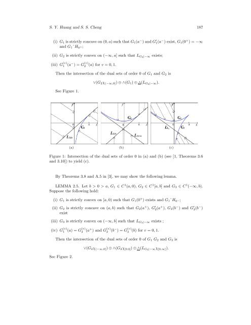
S. Y. Huang and S. S. Cheng 187
(i) G 1 is strictly concave on (0, a) such that G 1 (a − ) and G ′ 1(a − ) exist, G 1 (0 + ) = −∞
and G 1˜H 0 +;
(ii) G 2 is strictly convex on (−∞, a] such that L G2|−∞ exists;
(iii) G (v)
1 (a− ) = G (v)
2 (a) for v = 0, 1.
Then the intersection of the dual sets of order 0 of G 1 and G 2 is
See Figure 1.
∨(G 2 χ (−∞,0] ) ⊕ ∧(G 1 ) ⊕ ∧(L G2|−∞).
(a) (b) (c)
Figure 1: Intersection of the dual sets of order 0 in (a) and (b) (see [1, Theorems 3.6
and 3.10]) to yield (c).
By Theorems 3.8 and A.5 in [3], we may show the following lemma.
LEMMA 2.5. Let b > 0 > a, G 1 ∈ C 1 (a, 0), G 2 ∈ C 1 [a, b] and G 3 ∈ C 1 (−∞, b).
Suppose the following hold:
(i) G 1 is strictly convex on [a, 0) such that G 1 (0 + ) exists and G 1˜H 0 −;
(ii) G 2 is strictly concave on (a, b) such that G 2 (a + ), G ′ 2 (a+ ), G 2 (b − ) and G ′ 2 (b− )
exist
(iii) G 3 is strictly convex on (−∞, b] such that L G3|−∞ exists ;
(iv) G (v)
1 (a) = G(v) 2 (a+ ) and G (v)
2 (b− ) = G (v) (b) for v = 0, 1.
Then the intersection of the dual sets of order 0 of G 1 G 2 and G 3 is
See Figure 2.
∨(G 2 χ (−∞,0] ) ⊕ ∧(G 2 χ [0,b] ) ⊕ ∧(L G3|−∞χ [0,∞] ).
3