- Page 1 and 2: Evaluating dependability metrics of
- Page 3 and 4: Outline 1 Introduction 2 Monte Carl
- Page 5: Rare events Rare events occur when
- Page 8 and 9: Outline 1 Introduction 2 Monte Carl
- Page 10 and 11: Accuracy: how accurate is ¯X n ? W
- Page 12 and 13: A fundamental example: evaluating i
- Page 14 and 15: Other examples Reliability at t:
- Page 16 and 17: From the accuracy point of view, th
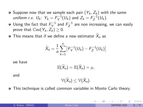
- Page 18 and 19: Variance reduction: antithetic vari
- Page 22 and 23: Variance reduction: control variabl
- Page 24: Monte Carlo drawbacks So, is there
- Page 27 and 28: What is crude simulation? Assume we
- Page 29 and 30: Inefficiency of crude Monte Carlo:
- Page 31 and 32: Robustness properties: Bounded rela
- Page 33 and 34: Relation between BRE and AO AO weak
- Page 35 and 36: Outline 1 Introduction 2 Monte Carl
- Page 37 and 38: Estimator and goal of IS Take (Y i
- Page 39 and 40: If A = [T, ∞), i.e., µ = P[Y ≥
- Page 41 and 42: IS for a discrete-time Markov chain
- Page 43 and 44: Zero-variance IS estimator for Mark
- Page 45 and 46: Zero-variance approximation Use a h
- Page 47 and 48: Drawbacks of the learning technique
- Page 49 and 50: Other procedure: optimization withi
- Page 51 and 52: Adaptive learning in Cross-Entropy
- Page 53 and 54: Splitting: general principle Splitt
- Page 55 and 56: Splitting and Markov chain {Y j ; j
- Page 57 and 58: The different implementations Fixed
- Page 59 and 60: Issues to be solved How to define t
- Page 61 and 62: Optimal values In a general setting
- Page 63 and 64: Simplified setting: fixed splitting
- Page 65 and 66: Illustration, fixed effort: a tande
- Page 67 and 68: Confidence interval issues Robustne
- Page 69 and 70: IS probability used Failure Biasing
- Page 71 and 72:
Asymptotic explanation When ε smal
- Page 73 and 74:
Tutorial on Monte Carlo techniques,
- Page 76 and 77:
• Very used in dependability anal
- Page 78 and 79:
• Usual situation: at some time s
- Page 80 and 81:
first order (in ε) expressions bef
- Page 82 and 83:
efore after a 1 a 2 x ε 2 ε 1 a 1
- Page 84 and 85:
symbolically, for an operational st
- Page 86 and 87:
• Always the same idea: take adva
- Page 88 and 89:
ε 1 ε 2 a 1 x a 2 before ε 4 ε
- Page 90 and 91:
• The zero variance idea in IS le
- Page 93 and 94:
• A variance-reduction procedure
- Page 95 and 96:
s t r 1 r 2 r 3 r 4 r 5 R st = r 1
- Page 97 and 98:
A COMMUNICATION NETWORK backbone, o
- Page 99 and 100:
A COMMUNICATION NETWORK • nodes a
- Page 101 and 102:
• Ω : set of all partial sub-gra
- Page 103 and 104:
• #failed = 0 • for m = 1, 2,
- Page 105 and 106:
• the correct answer given by the
- Page 107 and 108:
R = 1 R = r × R = r |K | = 1 |K |
- Page 109 and 110:
1 R r 2 = R r 1 r 2 R r 1 r 2 r 3 r
- Page 111:
1 R r 2 = R r 1 r 2 R r 1 r 5 etc.
- Page 117 and 118:
• Again, with P be a path and P-u
- Page 119 and 120:
- if the network is r 1 r 2 r 3 - t
- Page 121 and 122:
- then if the network is - then Z =
- Page 123 and 124:
• We partition Ω in the followin
- Page 125 and 126:
Ω = {L 1 L 2 , L 1 , L 1 L 2 } Z =
- Page 127 and 128:
Ω = {L 1 L 2 , L 1 , L 1 L 2 } Z =
- Page 129 and 130:
• It consists of generalizing thi
- Page 131 and 132:
Ω L 1 L’ 2 L’ 3 L 1 L 1 L’ 2
- Page 133 and 134:
L 1 L’ 2 L’ 3 L 1 L 1 L’ 2 L
- Page 135 and 136:
L 1 L’ 2 L’ 3 L 1 L 1 L’ 2 L
- Page 137 and 138:
L 1 L’ 2 L’ 3 L 1 L 1 L’ 2 L
- Page 139 and 140:
• sum = 0.0 • for m = 1, 2, …
- Page 141 and 142:
|V | = 9, |K | = 4, |E | = 12 M = 1
- Page 143 and 144:
• We varied K (|K | = 2, |K | = 5
- Page 145 and 146:
• We also varied r i = r from 0.9
- Page 148 and 149:
• A time-reduction procedure for
- Page 150 and 151:
• Internal loop: sampling a graph
- Page 152 and 153:
• We consider the case of case r
- Page 154 and 155:
• For a table with M rows, - each
- Page 156 and 157:
• Dividing the mean cost of the s
- Page 158:
• The procedure can be improved f
- Page 161:
• Reference: G. Rubino, B. Tuffin