David Thomas Hill PhD Thesis - Research@StAndrews:FullText ...

Chapter 1. Introduction: The luminosity distribution and total luminosity density of
galaxies
counts the number of galaxies with luminosity inside the range covered by the bin. The
H function weights each galaxy depending upon which bins it could fall within, and the
luminosity density present within those bins. It is therefore an iterative process, with each
repetition using the luminosity density values calculated in the previous iteration.
The key modification between the Efstathiou et al. and Norberg et al. methods is
the introduction of an individual magnitude limit (mlim,i) for each object. The Norberg
et al. method was also adopted by the 6dfGS and MGC (Jones et al., 2006; Driver et al.,
2005) teams for dealing with non-uniform flux limits. It also allows for the construction
of accurate luminosity distributions using bandpasses that did not define the limits of the
sample.
1.3.2 The Schechter Function
The shape of the luminosity distribution in the UV-NIR follows a similar pattern. As lu-
minosity decreases, the luminosity density increases exponentially, until a point is reached
where the rate of increase flattens, and the distribution follows a power-law like relation.
Attempts to parametrise the galaxy luminosity distribution began over half a century
ago. The current standard, the Schechter function (Schechter, 1976), built upon work by
Hubble (1936b) (who studied only the brightest galaxies and found a normally distributed
sample), Zwicky (1957) (who extended the work to faint dwarf galaxies and found an expo-
nential increase), Kiang (1961) and Abell (1958), amongst others. In terms of luminosity
it contains both power law and exponential components; when converted into magnitudes
it becomes a double exponential expression.
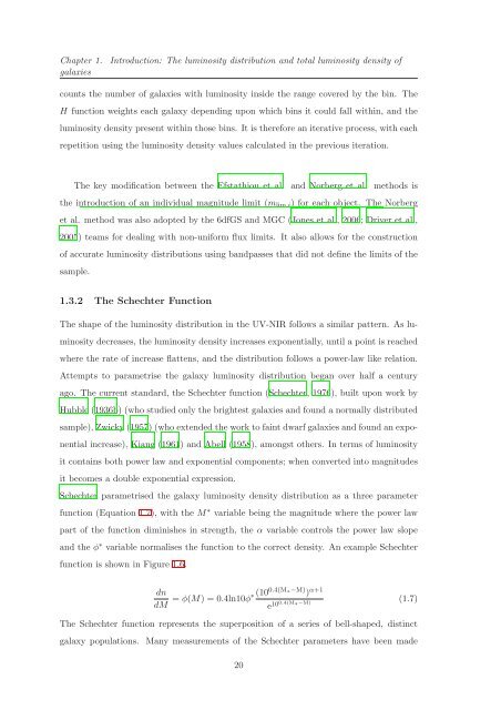
Schechter parametrised the galaxy luminosity density distribution as a three parameter
function (Equation 1.7), with the M ∗ variable being the magnitude where the power law
part of the function diminishes in strength, the α variable controls the power law slope
and the φ ∗ variable normalises the function to the correct density. An example Schechter
function is shown in Figure 1.6.
dn
dM = φ(M) = 0.4ln10φ∗(100.4(M∗−M) ) α+1
e100.4(M∗−M) (1.7)
The Schechter function represents the superposition of a series of bell-shaped, distinct
galaxy populations. Many measurements of the Schechter parameters have been made
20