Discrete Wavelet Transform-based Baseline Wandering ... - ijabme.org

INTERNATIONAL JOURNAL OF APPLIED BIOMEDICAL ENGINEERING VOL.3, NO.1 2010 27
It uses the wavelet function and scaling function to
analyze the signal of interest. In discrete wavelet
transform analysis, a given signal s(t) is decomposed
on multi-resolution levels as follows:
s (t) =
∞∑
k=−∞
c j (k)φ j,k (t) +
J∑
∞∑
j=1 k=−∞
d j (k)ψ j,k (t)
(1)
where ψ j,k (t) is the wavelet function and φ j,k (t) is the
scaling function. They are defined as
φ j,k (t) = 2 j/2 φ(2 j t − k) (2)
ψ j,k (t) = 2 j/2 ψ(2 j t − k) (3)
In wavelet analysis, dj(k) and cj(k) are computed by
using the filtering operation. dj(k) denotes the detailed
signals or wavelet coefficients and cj(k) represents
the approximated signals or scaling coefficients
at each level of decomposition. The DWT has the
capability of decomposing a signal of interest into an
approximation and detail information. It can thus
analyze the signal at different frequency ranges with
different resolutions. The DWT is implemented by
means of a pair of digital filter banks where the signal
is successively decomposed. The two filters are a
high pass filter and a low pass filter. Scaling function
and wavelet function are associated with low pass and
high pass filters, respectively, and they are used in the
DWT algorithm. These filters provide the decomposition
of the signal with different frequency bands by
recursively applying filters to the signal. The signal
is then split equally into its high and low frequency
components, called details and approximations, respectively.
In the DWT algorithm, the input signal
s(t) is first passed through the high pass filter and
low pass filter, and subsequently the outputs of both
filters are decimated by a factor of two. The input
signal to the filters is the HRECG. The high pass filtered
data set is the detail coefficients at level 1 and
the low pass filtered data set is the approximation
coefficients at level 1. This process can continue for
further decomposition at level 2,3,4, until the limit of
data length is reached. In addition, it is possible to
reconstruct the original signal from the approximation
and detail coefficients.
2.3 Data Analysis
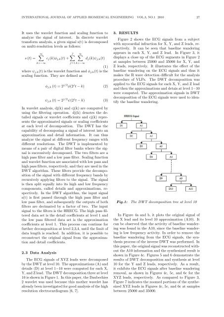
The ECG signals of XYZ leads were decomposed
by the DWT at level 10. The approximations (A) and
details (D) at level 1−10 were computed for each X,
Y, and Z lead. The DWT decomposition three at level
10 is shown in Figure 1. In this paper, the Daubechies
2 wavelet was used because this mother wavelet has
already been investigated for good analysis of the high
resolution electrocardiogram [6, 7].
3. RESULTS
Figure 2 shows the ECG signals from a subject
with myocardial infraction for X, Y, and Z leads, respectively.
It can be seen that baseline wandering
appears in each X, Y, and Z lead. In Figure 3, it
displays a close up of the ECG segments in Figure 2
at samples between 25000 and 35000 for X, Y, and
Z leads, respectively. It illustrates the effect of the
baseline wandering on the ECG signals and thus it
makes the R wave detection difficult for the analysis
procedure of VLPs. The DWT decomposition was
applied to the ECG signals for each X, Y, and Z lead
and then the approximations and detais at level 1−10
were computed. The approximation signals in DWT
decomposition of the ECG signals were used to identify
the baseline wandering.
Fig.1: The DWT decomposition tree at level 10
In Figure 4a and b, it plots the original signal of
the X lead and its level 10 approximation (A10). It
can be observed that the activity of baseline wandering
was found in the A10, since the baseline wandering
is low frequency activity. In order to remove the
baseline wandering from the ECG signals, the synthesis
process of the inverse DWT was performed. In
this paper, the original signal was reconstructed without
the A10 information and the synthesized result is
shown in Figure 4c. Figures 5 and 6 demonstrate the
results of DWT decomposition and synthesis at level
10 for the Y and Z leads, respectively. As a result,
it exhibits the ECG signals after baseline wandering
removal, as shown in Figures 4c, 5c, and 6c for the
XYZ leads, respectively. As compared to Figure 3,
Figure 7 indicates the zoomed portions of the synthesized
XYZ leads in Figures 4c, 5c, and 6c at samples
between 25000 and 35000.