Relay Approach for tuning of PID controller - International Journal of ...

Amar G Khalore et al ,Int.J.Computer Technology & Applications,Vol 3 (3), 1237-1242
ISSN:2229-6093
therefore be classified according to this experimental
procedure. The Tuning methods can be broadly
classified into the following categories where the
classification is based on the availability of the
process model and the model type.
2.1.1 Limit cycle method:
This method was proposed by Niederlinski
(1971) which is a more natural extension of the ZN
tuning procedure of the MIMO case. It is based on
replacing the controllers by gains and identifying a
critical point consisting of n scalar critical gains and
the critical frequency. The main departure from the
SISO case is that MIMO systems have infinitely
many critical points. The collection of these points
defines a hyper surface in the gains space called the
stability limit. Consequently, one has to prespecify
the desired critical point, e.g. equal loop gains. The
choice of the desired critical point depends on the
relative importance of the various loops, which is
commonly expressed through weighting factors.
Once the parameters of the critical point have been
determined, the controllers are tuned in a fashion
similar to the classical ZN rules, possibly with some
modifications. This method is briefly described
below:
(i) Choose n weighing factors ci (i = 1, 2 . . . n) for
the relative control quality of the n controlled
variables.
(ii) Using the best input output pairing bring the P -
controlled system to the stability limit keeping the
following relations between loop gains as
K . G C
K . G C
ci i, i(0)
i
ci 1 i 1, i 1(0) i 1
--------------------------- (2.1)
Where Kc, i is the gain of the P controller in the ith
loop and Gi,i are the diagonal process gains.
(iii) Determine the critical frequency wci from the
oscillation period Tu and the critical gain
Kui when the oscillations just commences with Kci at
Kui
(iv) Determine the controller parameters using the
Generalised Ziegler Nichols formulae listed in table
2.1 where the choice of coefficients αi depends on the
ratio
i
c
ci
.
Such that Ωc is the critical frequency when all the P-
controlled loops are active, whereas wci is the critical
frequency of the ith loop.
(v) Check whether the control quality is satisfactory.
If not change αi appropriately and return to step (ii).
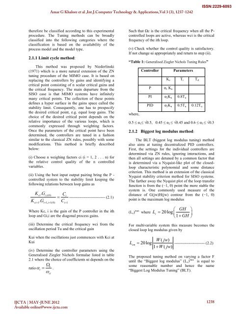
“Table 1: Generalised Ziegler Nichols Tuning Rules”
where,
Controller
P
Parameters
K c T i T d
α 1 K u
PI α 2 K u 0.8T u
PID α 3 K u 0.5T u 0.12T u
0.5 ≤ α 1 ≤ √0.5, 0.45 ≤ α 2 ≤ √0.45 and 0.6 ≤ α 3 ≤ √0.3
2.1.2 Biggest log modulus method:
The BLT (biggest log modulus tuning) method
also aims at tuning decentralized PID controllers.
First, the settings for the individual controllers are
determined via ZN rules, ignoring interactions, and
then all settings are detuned by a common factor that
is determined via a Nyquist-like plot of the closedloop
characteristic polynomial and some distance
criterion. This method is an extension of the classical
Nyquist stability criterion method for SISO systems.
The farther away the Nyquist plot of the loop transfer
function is from the (−1, 0) point the more stable the
system is. One commonly used measure of the
distance of G(jw)H(jw) contour from the (−1, 0)
point is the maximum log modulus
GH
(L c ) max where Lc
20log 1 GH
For multivariable system this measure becomes the
closed loop log modulus given by
L
cm
W ( jw)
20log 1 W ( jw )
----------------------- (2.2)
The proposed tuning method on varying a factor F
until the “Biggest log modulus” (L c ) max is equal to
some reasonable number and hence the name
“Biggest Log Modulus Tuning” (BLT).
IJCTA | MAY-JUNE 2012
Available online@www.ijcta.com
1238