Applications of Braid Theory
Applications of Braid Theory
Applications of Braid Theory

Create successful ePaper yourself
Turn your PDF publications into a flip-book with our unique Google optimized e-Paper software.
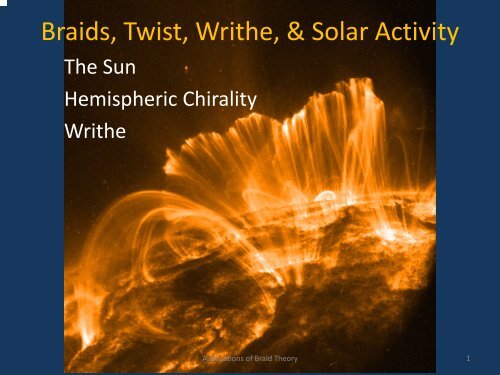
<strong>Braid</strong>s, Twist, Writhe, & Solar Activity<br />
The Sun<br />
Hemispheric Chirality<br />
Writhe<br />
<strong>Applications</strong> <strong>of</strong> <strong>Braid</strong> <strong>Theory</strong> 1
Coronal Heating<br />
Parker model (1983): The interior structure t re <strong>of</strong><br />
coronal loops is braided.<br />
When neighbouring tubes are misaligned by<br />
~ 30 degrees, reconnection removes a<br />
crossing, releasing magnetic energy into<br />
heat – a nan<strong>of</strong>lare.<br />
Linton, Dahlburg and Antiochos 2001<br />
<strong>Applications</strong> <strong>of</strong> <strong>Braid</strong> <strong>Theory</strong> 2
Hemispheric Chirality<br />
Sunspot whorls<br />
Filaments<br />
<strong>Applications</strong> <strong>of</strong> <strong>Braid</strong> <strong>Theory</strong> 3
Coronal Magnetic Structures <strong>of</strong>ten display kinked<br />
or helical structure ….<br />
Yohkoh s<strong>of</strong>t x-ray image<br />
<strong>of</strong> Southern hemisphere<br />
sigmoid<br />
X‐Ray Bi Brightenings i (Sigmoids) id
For closed curves and fields:<br />
Magnetic Helicity<br />
1. For two linked torii <strong>of</strong> flux F 1 and F 2 , and internal twists T 1 and T 2<br />
2. Helicity is an ideal MHD invariant.<br />
<strong>Applications</strong> <strong>of</strong> <strong>Braid</strong> <strong>Theory</strong> 5
Magnetic Helicity <strong>of</strong> a subvolume <strong>of</strong> space<br />
<strong>Applications</strong> <strong>of</strong> <strong>Braid</strong> <strong>Theory</strong> 6
global and regional helicities<br />
Let space be divided into N regions. Let H i be the helicity in region i (relative to vacuum<br />
field). Then for regions separated by parallel planes or concentric spheres,
Helicity between two planes can be expressed as a sum<br />
<strong>of</strong> winding numbers, over all pairs <strong>of</strong> field lines:
What if curves go up and down?<br />
1. Cut the curves into segments at turning points<br />
in height.<br />
2. Sum winding numbers for each<br />
pair <strong>of</strong> segments (if opposite<br />
directions, multiply by ‐1).<br />
Heresegments2and3give<br />
Here segments 2 and 3 give<br />
winding angle <strong>of</strong> ‐4p.
Solar Helicity Observations<br />
Current helicity j z /B z from vector magnetograms<br />
(Abramenko et al 1997; Pevtsov & Latushko 2002)<br />
Effects <strong>of</strong> differential rotation on active regions (van<br />
Ballegooijen et al 1998; B & Ruzmaikin 2000; Devore 2000; Green et al<br />
2002; Nindos et al 2003)<br />
Helicity flow through photosphere (Kusano et al 2002; Tian<br />
2003; Démoulin & B 2003; Chae et al 2004; Kusano et al 2005; Pariat et al<br />
2006; Longcope 2007)<br />
Magnetograms plus best‐fit force‐free free extrapolations<br />
(Démoulin et al 2002; Aulanier et al 2002, 2005)
Sigmoids<br />
S<strong>of</strong>t X‐ray brightenings g first<br />
identified in Yohkoh (Rust &<br />
Kumar 1996).<br />
Most (91%) active regions<br />
containing sigmoids also<br />
display filaments (Pevtsov<br />
2002).<br />
Sigmoids are mostly S shaped in the South and<br />
shaped in the North
Sigmoids are <strong>of</strong>ten precursors <strong>of</strong><br />
Coronal Mass Ejections
Flux Tube Models<br />
Twisted Flux tubes have <strong>of</strong>ten been used in models <strong>of</strong> solar<br />
filaments and Coronal Mass Ejections. Could the Sigmoid x‐ray<br />
brightenings show the shape <strong>of</strong> these tubes?<br />
Low & Berger 2003: magnetostatic solutions with<br />
helical symmetry embedded in external field<br />
Unfortunately, these give<br />
the wrong sign! However,<br />
surrounding current<br />
concentrations can have the<br />
correct sign.
Sideways helical tubes? No! the sign is<br />
wrong! shape for positive helicity<br />
– opposite to hemispheric law.
(2004, 2005)<br />
Kliem & Török simulation<br />
Follow nonlinear evolution <strong>of</strong> kink<br />
instability in Titov – Démoulin model<br />
‐‐‐ Intense currents develop along field<br />
Intense currents develop along field<br />
lines below flux tube which resemble<br />
sigmoids <strong>of</strong> the correct sign.
Gibson & Fan model
Linking, Twist, and Writhe<br />
Calugareanu 1961: Linking number = Twist + Writhe
For closed curves:<br />
Writhe
A trefoil knot and its tantrix curve<br />
Let A = the area enclosed by the tantrix curve.<br />
Then<br />
(Fuller 1971)
Writhe (by popular belief)<br />
Kink instability: internal twist converted to writhe<br />
(Ricca & M<strong>of</strong>fatt 1995, Rust 1996)<br />
Stretch‐Twist‐Fold Dynamos: large scale positive<br />
writhe helicity, small scale negative twist helicity<br />
(Gilbert 2003)<br />
Outer Convection Zone: coriolis force on rising<br />
tubes creates large scale positive writhe helicity,<br />
small scale negative twist helicity (in North)<br />
– ‘bihelical fields’ (Blackman & Brandenburg)<br />
– S effect (Longcope & Pevtsov): helicity source in active<br />
regions?
Helicity Decomposition<br />
Magnetic Helicity for (thin) closed flux tube with axial<br />
flux Φ:<br />
But how do we define the writhe <strong>of</strong> a curve with<br />
endpoints on a boundary plane (or boundary<br />
sphere)?
Answer: write the writhe <strong>of</strong> a framed curve as the<br />
difference between winding number and twist <strong>of</strong> the<br />
curves on the tube.<br />
When averaged over the<br />
tube, this is independent<br />
<strong>of</strong> framing.<br />
<strong>Applications</strong> <strong>of</strong> <strong>Braid</strong> <strong>Theory</strong> 22
This methods divides up a curve into pieces at its maxima and<br />
minima, then computes the “local writhe” <strong>of</strong> each piece<br />
(winding – twist), and the “nonlocal writhes” (just winding)<br />
between pieces. Total writhe = ‐0.752<br />
local writhe<br />
= 0.374<br />
Nonlocal writhe = ‐1.5<br />
local writhe<br />
= 0.374
Example: the tangent to a vertical helix has constant<br />
latitude<br />
The local writhe term equals the area<br />
The local writhe term equals the area<br />
between the tantrix curve and the North pole
Writhe can also be defined for loops by extending the<br />
loop and calculating the corresponding enclosed tantrix<br />
area (same results!)
Normal and Anomalous writhe<br />
How an elastic rod buckles:<br />
Normally,<br />
Negative twist S shape (as seen from above)<br />
Positive twist shape<br />
Solar sigmoids:<br />
Two positive twist sigmoids<br />
anomalous!
Kinked Loop: Sine Height pr<strong>of</strong>ile<br />
heig ght<br />
Sine height pr<strong>of</strong>ile z ∼ SinHπ tL<br />
0.4<br />
0.3<br />
0.2<br />
0.1<br />
0<br />
0 0.2 0.4 0.6 0.8 1<br />
horizontal position<br />
Twisted Sine Shape<br />
0.3<br />
0.2<br />
0.1<br />
Writh he<br />
0<br />
−0.1<br />
−0.2<br />
−0.3<br />
Q=-pê2<br />
Q=-3pê8<br />
Q=-pê4ê<br />
Q=-pê8<br />
0 0.2 0.4 0.6 0.8 1<br />
height Hunits <strong>of</strong> footpoint separationL<br />
h=0.4 Ө = ‐π/4
Two loops with identical Writhe = ‐0.2<br />
Normal<br />
Anomalous<br />
Sigmoids on the sun seem to be <strong>of</strong> the anomalous type