SCIRun Forward/Inverse ECG Toolkit - Scientific Computing and ...

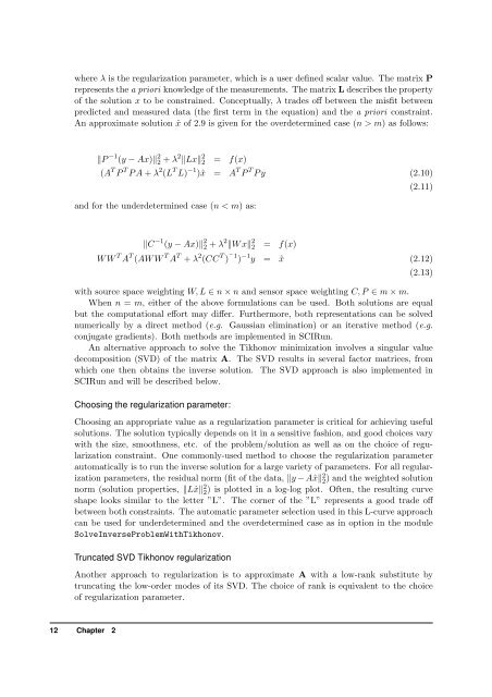
where λ is the regularization parameter, which is a user defined scalar value. The matrix P
represents the a priori knowledge of the measurements. The matrix L describes the property
of the solution x to be constrained. Conceptually, λ trades off between the misfit between
predicted and measured data (the first term in the equation) and the a priori constraint.
An approximate solution ˆx of 2.9 is given for the overdetermined case (n > m) as follows:
‖P −1 (y − Ax)‖ 2 2 + λ 2 ‖Lx‖ 2 2 = f(x)
(A T P T P A + λ 2 (L T L) −1 )ˆx = A T P T P y (2.10)
(2.11)
and for the underdetermined case (n < m) as:
‖C −1 (y − Ax)‖ 2 2 + λ 2 ‖W x‖ 2 2 = f(x)
W W T A T (AW W T A T + λ 2 (CC T ) −1 ) −1 y = ˆx (2.12)
(2.13)
with source space weighting W, L ∈ n × n and sensor space weighting C, P ∈ m × m.
When n = m, either of the above formulations can be used. Both solutions are equal
but the computational effort may differ. Furthermore, both representations can be solved
numerically by a direct method (e.g. Gaussian elimination) or an iterative method (e.g.
conjugate gradients). Both methods are implemented in SCIRun.
An alternative approach to solve the Tikhonov minimization involves a singular value
decomposition (SVD) of the matrix A. The SVD results in several factor matrices, from
which one then obtains the inverse solution. The SVD approach is also implemented in
SCIRun and will be described below.
Choosing the regularization parameter:
Choosing an appropriate value as a regularization parameter is critical for achieving useful
solutions. The solution typically depends on it in a sensitive fashion, and good choices vary
with the size, smoothness, etc. of the problem/solution as well as on the choice of regularization
constraint. One commonly-used method to choose the regularization parameter
automatically is to run the inverse solution for a large variety of parameters. For all regularization
parameters, the residual norm (fit of the data, ‖y − Aˆx‖ 2 2 ) and the weighted solution
norm (solution properties, ‖Lˆx‖ 2 2 ) is plotted in a log-log plot. Often, the resulting curve
shape looks similar to the letter ”L”. The corner of the ”L” represents a good trade off
between both constraints. The automatic parameter selection used in this L-curve approach
can be used for underdetermined and the overdetermined case as in option in the module
SolveInverseProblemWithTikhonov.
Truncated SVD Tikhonov regularization
Another approach to regularization is to approximate A with a low-rank substitute by
truncating the low-order modes of its SVD. The choice of rank is equivalent to the choice
of regularization parameter.
12 Chapter 2