Millikan writeup - Physics
Millikan writeup - Physics
Millikan writeup - Physics

Create successful ePaper yourself
Turn your PDF publications into a flip-book with our unique Google optimized e-Paper software.
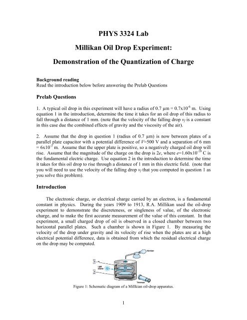
PHYS 3324 Lab<br />
<strong>Millikan</strong> Oil Drop Experiment:<br />
Demonstration of the Quantization of Charge<br />
Background reading<br />
Read the introduction below before answering the Prelab Questions<br />
Prelab Questions<br />
1. A typical oil drop in this experiment will have a radius of 0.7 µm = 0.7x10 -6 m. Using<br />
equation 1 in the introduction, determine the time it takes for an oil drop of this radius to<br />
fall through a distance of 1 mm. (note that the velocity of the falling drop v f is a constant<br />
in this case due the combined effects of gravity and the viscosity of the air).<br />
2. Assume that the drop in question 1 (radius of 0.7 µm) is now between plates of a<br />
parallel plate capacitor with a potential difference of V=500 V and a separation of 6 mm<br />
= 6x10 -3 m. Assume that the upper plate is positive, so a negatively charged oil drop will<br />
rise. Assume that the magnitude of the charge on the drop is 2e, where e=1.60x10 -19 C is<br />
the fundamental electric charge. Use equation 2 in the introduction to determine the time<br />
it takes for this oil drop to rise through a distance of 1 mm in this electric field. (note that<br />
you will need to use the velocity of the falling drop v f that you computed in question 1 as<br />
you solve this problem).<br />
Introduction<br />
The electronic charge, or electrical charge carried by an electron, is a fundamental<br />
constant in physics. During the years 1909 to 1913, R.A. <strong>Millikan</strong> used the oil-drop<br />
experiment to demonstrate the discreteness, or singleness of value, of the electronic<br />
charge, and to make the first accurate measurement of the value of this constant. In that<br />
experiment, a small charged drop of oil is observed in a closed chamber between two<br />
horizontal parallel plates. Such a chamber is shown in Figure 1. By measuring the<br />
velocity of the drop under gravity and its velocity of rise when the plates are at a high<br />
electrical potential difference, data is obtained from which the residual electrical charge<br />
on the drop may be computed.<br />
Figure 1: Schematic diagram of a Millkian oil-drop apparatus.<br />
1
The oil drops in the electric field between the plates are subject to three different<br />
forces: gravitational, electric and viscous (frictional or “drag” force between the air and<br />
oil). By analyzing these various forces, an expression can be derived which will enable<br />
measurement of the charge on the oil drop and determination of the unit charge on the<br />
electron.<br />
If m is the mass of the drop (sphere) under observation between the plates, the<br />
gravitational force on the drop is F g = mg. In the absence of any electric field, the only<br />
other force that acts is the viscous retarding force between the oil and the air; this force is<br />
given by F d = kv=6πηRv, where η is the coefficient of viscosity of the fluid (air) and R is<br />
the radius of the drop. The velocity of the drop quickly increases to the constant<br />
“terminal velocity” where these two forces are equal in magnitude F g = F d . This is<br />
shown in the left figure of Figure 2. So we have:<br />
F<br />
g<br />
mg F<br />
d<br />
6Rv<br />
f<br />
The mass of the spherical oil drop can be written in terms of the density ρ and radius R<br />
as m=(4/3)R 3 ρ. So, by measuring the fall velocity of the drop v f we can determine the<br />
radius of the drop by manipulating the above expression to give:<br />
9v<br />
f<br />
R (1)<br />
2g<br />
For parallel plates, a uniform electric field E=V/d can be generated by applying an<br />
electrical potential difference V across plates separated by a distance d. We will assume<br />
that the electric field is applied in such a direction that the force on a negatively charged<br />
particle will act upward (see right side of Figure 2). The combination of the three forces<br />
(gravity, viscous, and electrical) will cause the drop to rise with a constant velocity v r.<br />
The three forces combine to give zero net force:<br />
mg qE 6<br />
Rv 0<br />
r<br />
Figure 2: Left: No electric field; only gravitational and viscous forces act on the oil drop. Right: Electric<br />
field applied; gravitational, viscous, and electrical forces act on the oil drop.<br />
2
The above equation can be combined with equation 1 for the radius of the drop to give<br />
this expression for the charge on the drop (in terms of the measured fall and rise<br />
velocities – v f and v r ):<br />
v<br />
f 2 18d<br />
q v<br />
f<br />
vr<br />
<br />
3/<br />
(2)<br />
V 2g<br />
For a given oil drop, you will measure the fall time (T f ) in the absence of the electric field<br />
and the rise time (T r ) in the presence of the electric field over a fixed distance s. The fall<br />
and rise velocities can then be determined from v f = s/T f and v r = s/T r and the charge on<br />
the drop can be computed from Equation 2 above. (Note: all the quantities in equation 2<br />
are magnitudes, meaning they are all positive quantities. The signs were taken account of<br />
in the derivation of the equation.)<br />
Useful constants and data about our apparatus:<br />
d = separation of electric field capacitor plates = 6 mm = 6x10 -3 m<br />
ρ = density of the oil = 874 kg/m 3<br />
η = coefficient of viscosity of air = 1.81x10 -5 Ns/m 2<br />
g = acceleration due to gravity = 9.81 m/s 2<br />
e = accepted value of magnitude of the electron’s charge = 1.602x10 -19 C<br />
As always, when you are doing computations in this lab, it is very important to use a<br />
consistent set of units. Use SI units – meter for length, kilogram for mass, seconds for<br />
time, newtons for force, coulombs for charge, and volts for electric potential difference.<br />
3
Experimental Goal<br />
The goal of this experiment is to use the <strong>Millikan</strong> Oil Drop Apparatus to do the<br />
following:<br />
Demonstrate that electric charge only comes in discrete units – “ the quantization<br />
of charge”<br />
Measure the intrinsic charge of the electron (the smallest discrete unit of charge) e<br />
Figure 3: Desired output of the experiment – a histogram of the results of repeated measurements of the<br />
excess charge on oil drops. The histogram will clearly show the quantization of charge and allow a<br />
measurement of the elementary charge e.<br />
Apparatus<br />
First familiarize yourself with the apparatus. A diagram and picture of the apparatus<br />
as it should be set up for you are shown in Figure 4.<br />
Figure 4: The Leybold Didactic <strong>Millikan</strong> Oil Drop Apparatus<br />
4
Take a look at the apparatus and identify the following pieces:<br />
<br />
<br />
<br />
<br />
<br />
Two stopwatches: you will use these to measure the fall and rise time of each<br />
drop you study. The right button starts and stops the stop watch. The left button<br />
resets it.<br />
The <strong>Millikan</strong> power supply: this has no on/off switch. To bring it on plug in the<br />
connector from the power adapter to the 12 V in hole in the back. This supply<br />
does two things. It supplies to the power to the light (in the black housing on the<br />
stand that illuminates the oil drop chamber), and it applies the electric potential<br />
difference to the capacitor plates. There are two switches; put the switch labeled<br />
“t” in the down position and leave it that way for the whole lab – you won’t be<br />
using it.<br />
Take a look at the stand. You should see the <strong>Millikan</strong> oil drop chamber with its<br />
lucite housing (to reduce the effect of air currents). It has two metal capacitor<br />
plates separated by about 6 mm. There are also two small holes on the right hand<br />
side where oil drops can be admitted. Right by them is the atomizer, which is<br />
attached to a rubber bulb. By squeezing hard on the bulb, you force oil up<br />
through a capillary tube in the atomizer and a mist of oil droplet “spheres” is<br />
created.<br />
You should also see that there is a lamp on the right hand side (powered by the<br />
power supply) that shines light into the chamber. Note also that the chamber has<br />
black tape in the back – that is the dark background that you will view the bright<br />
oil droplets against. Finally, note that there is a telescope that you will use to<br />
actually view the droplets – more on that later.<br />
Verify that the connections from the power supply to the capacitor plates are<br />
hooked up so that the positive side (red lead) is on the top and the ground side<br />
(blue lead) is on the bottom.<br />
Turn the “U” switch to on and dial the voltage knob over its full range (0 – 600<br />
V). Then set it to 500 V (within ~ +/- 5 V or so). Leave it at that setting for the<br />
remainder of the lab. Turn the U knob off for now.<br />
Procedure<br />
1. First you will get use to viewing the oil drops and observe their general behavior.<br />
Look into the eyepiece. You should be able to see a vertical micrometer scale and a<br />
black background (the tape at the back of the chamber). The eyepiece has knob you can<br />
turn to adjust the focus on the micrometer scale; optimize it for your eye. Now squeeze<br />
on the atomizer rubber bulb. You may need to adjust the glass oil holder so its output is<br />
centered over the small holes on the right side of the chamber. You can vary the distance<br />
of this output from the side of the chamber to try to optimize the number of droplets you<br />
get in the chamber at a given time. You should be able to see small bright droplets in the<br />
chamber now. You can adjust the objective lens on the microscope using the rotary knob<br />
on its two sides. This will focus on different parts of the chamber, so you will see some<br />
droplets come into focus while others go out of focus. Finally, if needed you can adjust<br />
the postion of the light bulb relative to the chamber by loosening the screw on top that<br />
5
holds it in place. We tried to optimize it position beforehand, but feel free to adjust it if<br />
you want to try to vary the lighting of the interior of the chamber.<br />
2. Before doing anything quantitative, notice some general features of the behavior of the<br />
droplet. First, it is important to note that the microscope’s objective lens inverts the<br />
image. So if a drop is falling, you will see it rise in your image. Conversely, if a drop is<br />
rising you will see it falling in your image.<br />
<br />
<br />
<br />
First look at the droplets with no voltage applied to the capacitor plates. You<br />
should see them mostly rising (although some large ones may be nearly<br />
stationary). Since they appear to be rising, they are actually falling under the<br />
influence of gravity.<br />
Now turn on the voltage to the capacitor plates (500 V). You will see some<br />
drops slow down and some will actually reverse direction (meaning they are<br />
actually rising). These are droplets with an excess negative charge that are<br />
attracted to the top plate of the capacitor. So they either slow the rate of fall of<br />
the drop or reverse it and start rising if the residual negative charge is large<br />
enough.<br />
On the other hand, you will see some droplets actually start to fall faster (or rise<br />
faster as you actually see it). These are positively charged drops that are attracted<br />
electrically to the bottom plate of the capacitor (ie. the force on them is the same<br />
direction as the gravitational force).<br />
3. Now you are ready to do some quantitative measurements. The first thing to note is<br />
the calibration of the scale. The objective lens of the microscope has a magnification of<br />
2.00 and the eyepiece lens has a magnification of 10. So that means that the smallest<br />
division you see on the micrometer scale corresponds to a length of .05 mm. The<br />
distance between major scale divisions (which each have 10 minor divisions between<br />
them) is 0.5 mm. For convenience, all of your measurements should be done over the<br />
same vertical fall distance – 20 minor scale divisions (which is the same as two major<br />
scale divisions). That corresponds to a real vertical distance that the drop falls through of<br />
1.0 mm. You won’t need to worry in detail about this number until you do your report.<br />
4. For the quantitative part of the lab, you will just focus on negatively charged drops.<br />
Those are the ones that appear to be rising (actually falling) with 0V applied, and then<br />
when you apply 500 V, they reverse direction and appear to be falling (actually rising).<br />
For each droplet you select, you want to measure the time it takes to fall through 20<br />
minor scale divisions and the time it takes to rise through 20 minor scale divisions. For<br />
your report, you will use those two numbers to determine the radius of each drop and the<br />
charge on it.<br />
5. Prepare a table with columns for “Fall time” and “Rise time”. To be clear – fall time is<br />
the time with 0 V applied, so you will actually see the drop rising. Rise time is the time<br />
with 500 V applied, so you will actually see the drop falling. You are going to want to<br />
get a fall time and a rise time for a total of 30 drops. One partner should view the drops<br />
6
while the other runs the stopwatches. Each partner should get a chance to view drops (for<br />
2 partners each should view 15 apiece, for 3 partners each should view 10 apiece).<br />
6. Here is the recommended procedure for taking data for a drop:<br />
Set the U switch to ON (for 500 V applied)<br />
Squeeze the bulb to put a puff of drops in the chamber<br />
Locate a drop that appears to be going down (actually it is rising) and focus the<br />
objective lens on it<br />
Flip the switch to 0 V and 500 V back and forth to make sure you really have a<br />
drop that is reversing direction and that you have isolated on it.<br />
Now that you have “control” of the drop, set U to 0V and measure the time it<br />
takes to fall (it will appear to be rising) through 20 minor scale divisions (2 major<br />
scale divisions).<br />
Then flip the switch to on to apply 500 V and measure the time it takes to rise<br />
(it will appear to be falling) through 20 minor scale divisions (2 major scale<br />
divisions).<br />
Record your two times, reset the stopwatches, put another puff of droplets in the<br />
chamber, and look for a new drop to measure.<br />
7. Here are some typical ranges of times you should expect to use as a guide:<br />
<br />
<br />
Fall times: Fall times can be in the range of 5 – 40 seconds, with the bigger<br />
drops falling faster. Most of the fall times will be in the range 20-30 seconds, but<br />
if you occasionally see a fast one (5-10 seconds) try to take data on it so you have<br />
looked at a range of droplets.<br />
Rise time: Rise times can be seen over a somewhat wider range 5 – 70 seconds;<br />
once again try to get a range of values. The faster rise times typically correspond<br />
to drops with more charge on them.<br />
8. Before you leave lab, make sure you have a table with 30 values of fall and rise times<br />
for 30 different oil drops.<br />
Report<br />
Make sure your report for this lab includes all of the following:<br />
1. Introduction<br />
2. Qualitative description of droplet behavior: During the lab (in procedure step 2)<br />
you made some qualitative observations of the behavior of the droplets. Briefly describe<br />
what you observed when:<br />
<br />
<br />
you viewed the droplets with no electric field applied (V = 0 volts)<br />
you viewed the droplets with an electric field applied (V = 500 volts); you<br />
should have seen drops going both directions – explain that behavior<br />
7
3. Equations: Prepare the equations you will need to analyze your data. For each of<br />
your 30 droplet measurements, you should have recorded the “fall time” T f (time to fall<br />
under gravity alone with no electric field applied – V = 0 volts) and the “rise time” T r<br />
(time for negatively charged particles to rise in an applied electric field with V = 500<br />
volts). These times were to be measured over a fixed distance of 20 minor scale<br />
divisions. The calibration of the minor scale divisions was .05 mm per division (note: an<br />
earlier version of the lab <strong>writeup</strong> had an incorrect number for this). So over 20 divisions<br />
a distance of 1 mm = 1.0x10 -3 m was covered. (This is the “fixed distance” referred to as<br />
s on page 3 in the introduction to this lab). Start with equations (1) and (2) in the<br />
introduction to get the following two formulae in a form that will be useful to you:<br />
<br />
<br />
Radius: Plug in all the known constants to determine a formula for the radius<br />
of the droplets that only involves the fall time T f and a numerical constant.<br />
Charge: Plug in all the known constants to determine a formula for the charge<br />
(normalized to the accepted charge) q/e that only involves the fall and rise<br />
times T f and T r and a numerical constant.<br />
4. Data and calculations table: Make a single table for your 30 droplets with the<br />
following columns:<br />
Fall time in seconds<br />
Rise time in seconds<br />
Calculated value of the radius of the drop ( in units of micrometers = 1 µm =<br />
1.0x10 -6 m<br />
Calculated value of the charge (divided by the accepted value of the charge e):<br />
q/e<br />
“Corrected” value of the charge. It turns out that there are deviations from<br />
Stoke’s law (see introduction page 2) for the viscous retarding force between the<br />
droplets and the air when the droplets become as small as the ones we are using in<br />
this experiment. That is because the size of the droplets starts to become<br />
comparable to the mean free path between the air atoms. There is an empirical<br />
correction to to correct for this effect known as “Cunningham’s law”. It was<br />
applied by <strong>Millikan</strong> to his own data. It leads to a formula for the corrected value<br />
of the charge based on the observed radius of the drop. It is given as:<br />
q corrected<br />
q<br />
<br />
.07776m<br />
<br />
1 <br />
R <br />
3<br />
2<br />
where R is the radius of the drop. Apply this correction factor to each of your 30<br />
drops and put the result in a column of “Corrected q/e”<br />
Before exporting this table from your spreadsheet program, make sure to sort it<br />
based on this last column, so your data is sorted from the smallest value of<br />
“Correct q/e” to the largest.<br />
8
5. Plots: The best way to display your data is to make histograms of it.<br />
Histograms are plots of the frequency of occurrence of a particular quantity. You<br />
can generate histograms using any plotting package you prefer, but if you use<br />
Excel, you can find instructions for how to do it at:<br />
http://www.ncsu.edu/labwrite/res/gt/gt-bar-home.html#cb1<br />
For your 30 drops, make a histogram of the droplet radii and of your values of<br />
“Corrected” q/e.<br />
6. Extracted value of the fundamental charge: Look at your “Corrected q/e”<br />
values in your table and in your histogram. If your data was taken properly, you<br />
should see clusters of data near 1, 2, 3 (and maybe even 4, although that is rare)<br />
times the fundamental charge. Make an estimate of where the “dividing lines” are<br />
between these groups, and then for each group compute the average, standard<br />
deviation, and standard error of the mean. Record this information in a small<br />
table that includes the average, standard error of the mean, standard deviation, and<br />
number of points in that group. Now take the value of the charge from each<br />
group, divide by the number of charges (1,2,3, …) so you report an average value<br />
of the charge (and its error) as determined from each group. To determine your<br />
final value of the charge you need to take the weighted average of these numbers<br />
(and determine its error).<br />
7. Analysis with more data: On the “Calendar of Sessions” page of the lab<br />
website there is a link to “<strong>Millikan</strong> Data”. Download the Excel file there. It has<br />
some data taken using our apparatus with a large number of drops (159 in all).<br />
Do the same analysis as you did on the other data (but you don’t need to put in a<br />
complete data table for this one). Put the following into your report for this data:<br />
<br />
<br />
<br />
Histogram of the droplet radii<br />
Histogram of the corrected values of the charge (q/e)<br />
Group the data into charge groups and then go through the same steps<br />
from item 6 for this data; include the small summary table and final value<br />
of the charge (q/e) and its error<br />
8. Conclusion: Make sure your conclusion includes your conclusions about the goals:<br />
Demonstration of charge quantization<br />
Measurement of the intrinsic unit of charge – report both the final result from<br />
your 30 drop measurement and the result from the larger 159 drop data set<br />
If your q/e value is not equal to 1 within your measured errors, then make a<br />
comment about why not. There is a systematic error that we did not include here.<br />
Do you know what it is?<br />
9