MULTIVARIATE POLYNOMIALS IN SAGE
MULTIVARIATE POLYNOMIALS IN SAGE
MULTIVARIATE POLYNOMIALS IN SAGE

Create successful ePaper yourself
Turn your PDF publications into a flip-book with our unique Google optimized e-Paper software.
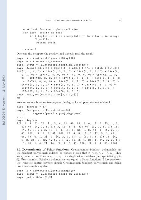
MULTIVARIABLE <strong>POLYNOMIALS</strong> <strong>IN</strong> <strong>SAGE</strong> 15<br />
# we look for the right coefficient<br />
for (key , coeff ) in res :<br />
if ([ key [i] for i in xrange (n)] == [n-i for i in xrange<br />
(1 ,n +1) ]):<br />
return coeff<br />
hal-00824143, version 1 - 21 May 2013<br />
return 0<br />
One can also compute the product and directly read the result:<br />
sage : A = AbstractPolynomialRing (QQ)<br />
sage : m = A. monomial _ basis ()<br />
sage : Schub = A. schubert _ basis _on_ vectors ()<br />
sage : Schub ( (3* m [1] + 2*m[0 ,1] + m [0 ,0 ,1]) ^4 * Schub [1 ,0 ,1 ,0])<br />
8*Y(1 , 1, 4, 0) + 23* Y(1 , 2, 3, 0) + 24* Y(1 , 3, 2, 0) + 39* Y(1 ,<br />
4, 1, 0) + 15* Y(1 , 5, 0, 0) + Y(1 , 0, 5, 0) + 48* Y(2 , 1, 3,<br />
0) + 101* Y(2 , 2, 2, 0) + 117* Y(2 , 3, 1, 0) + 84* Y(2 , 4, 0, 0)<br />
+ 12* Y(2 , 0, 4, 0) + 173* Y(3 , 1, 2, 0) + 78* Y(3 , 2, 1, 0) +<br />
147* Y(3 , 3, 0, 0) + 53* Y(3 , 0, 3, 0) + 283* Y(4 , 1, 1, 0) +<br />
171* Y(4 , 2, 0, 0) + 96* Y(4 , 0, 2, 0) + 93* Y(5 , 1, 0, 0) +<br />
176* Y(5 , 0, 1, 0) + 80* Y(6 , 0, 0, 0)<br />
sage : proj _ deg ( Permutation ([2 ,1 ,4 ,3]) )<br />
78<br />
We can use our function to compute the degree for all permutations of size 4:<br />
sage : degrees = {}<br />
sage : for perm in Permutations (4) :<br />
....: degrees [ perm ] = proj _ deg ( perm )<br />
....:<br />
sage : degrees<br />
{[2 , 1, 4, 3]: 78 , [1 , 3, 4, 2]: 48 , [3 , 2, 4, 1]: 3, [3 , 1, 2,<br />
4]: 48 , [4 , 2, 1, 3]: 3, [1 , 4, 2, 3]: 46 , [3 , 2, 1, 4]: 16 ,<br />
[4 , 1, 3, 2]: 3, [2 , 3, 4, 1]: 6, [3 , 4, 2, 1]: 1, [1 , 2, 3,<br />
4]: 720 , [1 , 3, 2, 4]: 280 , [2 , 4, 3, 1]: 3, [2 , 3, 1, 4]:<br />
46 , [3 , 4, 1, 2]: 2, [4 , 2, 3, 1]: 1, [1 , 4, 3, 2]: 16 , [4 ,<br />
1, 2, 3]: 6, [2 , 4, 1, 3]: 12 , [4 , 3, 1, 2]: 1, [4 , 3, 2, 1]:<br />
1, [3 , 1, 4, 2]: 14 , [2 , 1, 3, 4]: 220 , [1 , 2, 4, 3]: 220}<br />
4.2. Determinants of Schur functions. Grassmannian Schubert polynomials are<br />
the Schubert polynomials indexed by vectors v such that v 1 ≤ v 2 ≤ . . . ≤ v n . They<br />
are symmetric functions in x 1 , . . . , x n . In a single set of variables (i.e., specializing y to<br />
0), Grassmannian Schubert polynomials are equal to Schur functions. More precisely,<br />
the transition matrix between double Grassmannian Schubert polynomials and Schur<br />
functions is unitriangular.<br />
sage : A = AbstractPolynomialRing (QQ)<br />
sage : Schub = A. schubert _ basis _on_ vectors ()<br />
sage : pol = Schub [1 ,2]