The Cost of Future Collisions in LEO - Star Technology and Research
The Cost of Future Collisions in LEO - Star Technology and Research
The Cost of Future Collisions in LEO - Star Technology and Research

You also want an ePaper? Increase the reach of your titles
YUMPU automatically turns print PDFs into web optimized ePapers that Google loves.
18<br />
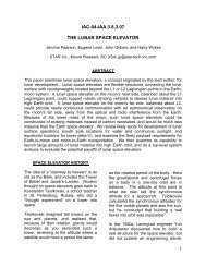
Fig. 10. <strong>The</strong> virtual stream <strong>and</strong> collision events.<br />
τ c , formula (41) turns <strong>in</strong>to (17), as expected, because it reflects accumulation <strong>of</strong><br />
the collision probability with time. Fig. 10 illustrates the relation between the<br />
growth <strong>of</strong> the average virtual stream (41) <strong>and</strong> a particular realization <strong>of</strong> the collision<br />
process. Virtual streams can also be evaluated as averages <strong>of</strong> many simulation runs<br />
<strong>in</strong> numerical models <strong>of</strong> the debris environment [1,2,10].<br />
Accord<strong>in</strong>g to formula (41), the fragments <strong>in</strong> the average virtual stream are<br />
produced at a constant rate (42). In a small period <strong>of</strong> time dτ, the fragment density<br />
is <strong>in</strong>creased by dρ = Udτ. Once created, the fragments start migrat<strong>in</strong>g down at the<br />
rates proportional to the air density at their altitudes. After time τ at an altitude<br />
H, we will see fragments from all layers between H <strong>and</strong> H τ , where H τ is def<strong>in</strong>ed by<br />
the solution <strong>of</strong> equation (37) with the <strong>in</strong>itial altitude H. Tak<strong>in</strong>g <strong>in</strong>to account the<br />
density scal<strong>in</strong>g rule (35) <strong>and</strong> disregard<strong>in</strong>g the radius variation between the layers,<br />
we f<strong>in</strong>d that<br />
ρ τ (m, H) ≈<br />
∫ τ<br />
0<br />
Ḣ t<br />
Ḣ U(m, H t) d˜t =<br />
∫<br />
1<br />
Hτ<br />
U(m, h) dh, (43)<br />
λt y ρ a (H) H<br />
where ˜t = t/t y is time <strong>in</strong> years, <strong>and</strong> t y is a period <strong>of</strong> one year. Integration yields<br />
1 ∑<br />
ρ τ ≈<br />
P ki f ki (m) [G ki (H) − G ki (H τ )], (44)<br />
λt y ρ a (H)<br />
k,i<br />
where G ki (H) is the cumulative distribution by altitude (9), which can be applied<br />
<strong>in</strong> a particular form <strong>of</strong> (15).<br />
Transition<strong>in</strong>g to the average flux, as we transitioned from (17) to (21), we<br />
derive the follow<strong>in</strong>g formula for the average virtual flux <strong>of</strong> fragments heavier than<br />
m, adjusted for the orbital decay due to air drag,<br />
Φ n ≈<br />
k n<br />
λt y ρ a (H)<br />
∑<br />
β nk P ki F ki (m) [G ki (H) − G ki (H τ )], (45)<br />
k,i<br />
where the coefficient k n has the same mean<strong>in</strong>g as <strong>in</strong> formula (21).<br />
To account for the variability <strong>of</strong> the ballistic coefficients <strong>of</strong> the fragments [11],<br />
we use a statistical average<br />
Φ a =<br />
∫ ∞<br />
0<br />
Φ n n(b c ) db c , (46)