- Page 3 and 4:
With WileyPLUS: This online teachin
- Page 5:
6 TH EDITION Business Statistics Fo
- Page 8 and 9:
Vice President & Publisher George H
- Page 10 and 11:
BRIEF CONTENTS UNIT I UNIT II UNIT
- Page 12 and 13:
x Contents 3.5 Descriptive Statisti
- Page 14 and 15:
xii Contents Statistical Hypotheses
- Page 16 and 17:
xiv Contents Forward Selection 572
- Page 19 and 20:
PREFACE The sixth edition of Busine
- Page 21 and 22:
Preface xix all of the inferential
- Page 23 and 24:
Preface xxi very limited access to
- Page 25 and 26:
Preface xxiii Interpreting the Outp
- Page 27:
Preface xxv ACKNOWLEDGMENTS John Wi
- Page 31 and 32:
UNIT I INTRODUCTION The study of bu
- Page 33 and 34:
Statistics Describe the State of Bu
- Page 35 and 36:
1.2 Basic Statistical Concepts 5 In
- Page 37 and 38:
1.3 Data Measurement 7 FIGURE 1.1 P
- Page 39 and 40:
1.3 Data Measurement 9 In addition,
- Page 41 and 42:
1.3 Data Measurement 11 Statistical
- Page 43 and 44:
Analyzing the Databases 13 1.3 Give
- Page 45 and 46:
Case 15 ASSIGNMENT Use the database
- Page 47 and 48:
Energy Consumption Around the World
- Page 49 and 50:
2.1 Frequency Distributions 19 TABL
- Page 51 and 52:
2.2 Quantitative Data Graphs 21 cla
- Page 53 and 54:
2.2 Quantitative Data Graphs 23 FIG
- Page 55 and 56:
2.2 Quantitative Data Graphs 25 FIG
- Page 57 and 58:
2.3 Qualitative Data Graphs 27 2.9
- Page 59 and 60:
2.3 Qualitative Data Graphs 29 FIGU
- Page 61 and 62:
2.3 Qualitative Data Graphs 31 STAT
- Page 63 and 64:
2.4 Graphical Depiction of Two-Vari
- Page 65 and 66:
Problems 35 Pie Charts for World Oi
- Page 67 and 68:
Supplementary Problems 37 2.19 Cons
- Page 69 and 70:
Supplementary Problems 39 include t
- Page 71 and 72:
Using the Computer 41 In 1983, the
- Page 73 and 74:
Using the Computer 43 ■ ■ ■ t
- Page 76 and 77:
CHAPTER 3 Descriptive Statistics LE
- Page 78 and 79:
48 Chapter 3 Descriptive Statistics
- Page 80 and 81:
50 Chapter 3 Descriptive Statistics
- Page 82 and 83:
52 Chapter 3 Descriptive Statistics
- Page 84 and 85:
54 Chapter 3 Descriptive Statistics
- Page 86 and 87:
56 Chapter 3 Descriptive Statistics
- Page 88 and 89:
ƒ ƒ 58 Chapter 3 Descriptive Stat
- Page 90 and 91:
60 Chapter 3 Descriptive Statistics
- Page 92 and 93:
62 Chapter 3 Descriptive Statistics
- Page 94 and 95:
64 Chapter 3 Descriptive Statistics
- Page 96 and 97:
66 Chapter 3 Descriptive Statistics
- Page 98 and 99:
68 Chapter 3 Descriptive Statistics
- Page 100 and 101:
70 Chapter 3 Descriptive Statistics
- Page 102 and 103:
72 Chapter 3 Descriptive Statistics
- Page 104 and 105:
74 Chapter 3 Descriptive Statistics
- Page 106 and 107:
76 Chapter 3 Descriptive Statistics
- Page 108 and 109:
78 Chapter 3 Descriptive Statistics
- Page 110 and 111:
80 Chapter 3 Descriptive Statistics
- Page 112 and 113:
82 Chapter 3 Descriptive Statistics
- Page 114 and 115:
84 Chapter 3 Descriptive Statistics
- Page 116 and 117:
86 Chapter 3 Descriptive Statistics
- Page 118 and 119:
88 Chapter 3 Descriptive Statistics
- Page 120 and 121:
90 Chapter 3 Descriptive Statistics
- Page 122 and 123:
CHAPTER 4 Probability LEARNING OBJE
- Page 124 and 125:
94 Chapter 4 Probability FIGURE 4.1
- Page 126 and 127:
96 Chapter 4 Probability Subjective
- Page 128 and 129:
98 Chapter 4 Probability FIGURE 4.3
- Page 130 and 131:
100 Chapter 4 Probability THE mn CO
- Page 132 and 133:
102 Chapter 4 Probability FIGURE 4.
- Page 134 and 135:
104 Chapter 4 Probability TABLE 4.2
- Page 136 and 137:
106 Chapter 4 Probability By the ge
- Page 138 and 139:
108 Chapter 4 Probability P (neithe
- Page 140 and 141:
110 Chapter 4 Probability 4.10 Use
- Page 142 and 143:
ƒ ƒ 112 Chapter 4 Probability ran
- Page 144 and 145:
114 Chapter 4 Probability DEMONSTRA
- Page 146 and 147:
116 Chapter 4 Probability 4.21 A st
- Page 148 and 149:
ƒ 118 Chapter 4 Probability The se
- Page 150 and 151:
ƒ 120 Chapter 4 Probability STATIS
- Page 152 and 153:
122 Chapter 4 Probability the South
- Page 154 and 155:
124 Chapter 4 Probability TABLE 4.8
- Page 156 and 157:
126 Chapter 4 Probability Event Pri
- Page 158 and 159:
128 Chapter 4 Probability ETHICAL C
- Page 160 and 161:
130 Chapter 4 Probability TESTING Y
- Page 162 and 163:
132 Chapter 4 Probability 4.49 In a
- Page 165 and 166:
UNIT II DISTRIBUTIONS AND SAMPLING
- Page 167 and 168:
Life with a Cell Phone As early as
- Page 169 and 170:
5.2 Describing a Discrete Distribut
- Page 171 and 172:
5.2 Describing a Discrete Distribut
- Page 173 and 174:
5.3 Binomial Distribution 143 5.3 T
- Page 175 and 176:
5.3 Binomial Distribution 145 selec
- Page 177 and 178:
5.3 Binomial Distribution 147 DEMON
- Page 179 and 180:
ƒ 5.3 Binomial Distribution 149 TA
- Page 181 and 182:
5.3 Binomial Distribution 151 FIGUR
- Page 183 and 184:
Problems 153 5.8 Use the probabilit
- Page 185 and 186:
5.4 Poisson Distribution 155 time i
- Page 187 and 188:
5.4 Poisson Distribution 157 Soluti
- Page 189 and 190:
5.4 Poisson Distribution 159 FIGURE
- Page 191 and 192:
5.4 Poisson Distribution 161 The Po
- Page 193 and 194:
Problems 163 data set as a basis fo
- Page 195 and 196:
5.5 Hypergeometric Distribution 165
- Page 197 and 198:
Problems 167 5.5 PROBLEMS 5.27 Comp
- Page 199 and 200:
Key Terms 169 problem, but it can b
- Page 201 and 202:
Supplementary Problems 171 5.36 Use
- Page 203 and 204:
Supplementary Problems 173 Suppose
- Page 205 and 206:
Case 175 ANALYZING THE DATABASES se
- Page 207 and 208:
Using the Computer 177 ■ in a col
- Page 209 and 210:
The Cost of Human Resources What is
- Page 211 and 212:
6.1 The Uniform Distribution 181 FI
- Page 213 and 214:
6.1 The Uniform Distribution 183 DE
- Page 215 and 216:
6.2 Normal Distribution 185 FIGURE
- Page 217 and 218:
6.2 Normal Distribution 187 TABLE 6
- Page 219 and 220:
6.2 Normal Distribution 189 This pr
- Page 221 and 222:
6.2 Normal Distribution 191 The pro
- Page 223 and 224:
6.2 Normal Distribution 193 DEMONST
- Page 225 and 226:
Problems 195 6.9 According to the I
- Page 227 and 228:
6.3 Using the Normal Curve to Appro
- Page 229 and 230:
6.3 Using the Normal Curve to Appro
- Page 231 and 232:
Problems 201 The answer obtained by
- Page 233 and 234:
6.4 Exponential Distribution 203 FI
- Page 235 and 236:
Problems 205 TABLE 6.6 Excel and Mi
- Page 237 and 238:
Summary 207 The area associated wit
- Page 239 and 240:
Supplementary Problems 209 6.36 Wor
- Page 241 and 242:
Supplementary Problems 211 availabi
- Page 243 and 244:
Using the Computer 213 that sales a
- Page 246 and 247:
CHAPTER 7 Sampling and Sampling Dis
- Page 248 and 249:
218 Chapter 7 Sampling and Sampling
- Page 250 and 251:
220 Chapter 7 Sampling and Sampling
- Page 252 and 253:
222 Chapter 7 Sampling and Sampling
- Page 254 and 255:
224 Chapter 7 Sampling and Sampling
- Page 256 and 257:
226 Chapter 7 Sampling and Sampling
- Page 258 and 259:
228 Chapter 7 Sampling and Sampling
- Page 260 and 261:
230 Chapter 7 Sampling and Sampling
- Page 262 and 263:
232 Chapter 7 Sampling and Sampling
- Page 264 and 265:
234 Chapter 7 Sampling and Sampling
- Page 266 and 267:
236 Chapter 7 Sampling and Sampling
- Page 268 and 269:
238 Chapter 7 Sampling and Sampling
- Page 270 and 271:
240 Chapter 7 Sampling and Sampling
- Page 272 and 273:
242 Chapter 7 Sampling and Sampling
- Page 274 and 275:
244 Chapter 7 Sampling and Sampling
- Page 276 and 277:
246 Chapter 7 Sampling and Sampling
- Page 278 and 279:
248 Making Inferences About Populat
- Page 280 and 281:
CHAPTER 8 Statistical Inference: Es
- Page 282 and 283:
252 Chapter 8 Statistical Inference
- Page 284 and 285:
254 Chapter 8 Statistical Inference
- Page 286 and 287:
256 Chapter 8 Statistical Inference
- Page 288 and 289:
258 Chapter 8 Statistical Inference
- Page 290 and 291:
260 Chapter 8 Statistical Inference
- Page 292 and 293:
262 Chapter 8 Statistical Inference
- Page 294 and 295:
264 Chapter 8 Statistical Inference
- Page 296 and 297:
266 Chapter 8 Statistical Inference
- Page 298 and 299:
268 Chapter 8 Statistical Inference
- Page 300 and 301:
270 Chapter 8 Statistical Inference
- Page 302 and 303:
272 Chapter 8 Statistical Inference
- Page 304 and 305:
274 Chapter 8 Statistical Inference
- Page 306 and 307:
276 Chapter 8 Statistical Inference
- Page 308 and 309:
278 Chapter 8 Statistical Inference
- Page 310 and 311:
280 Chapter 8 Statistical Inference
- Page 312 and 313:
282 Chapter 8 Statistical Inference
- Page 314 and 315:
284 Chapter 8 Statistical Inference
- Page 316:
286 Chapter 8 Statistical Inference
- Page 319 and 320:
Word-of-Mouth Business Referrals an
- Page 321 and 322:
9.1 Introduction to Hypothesis Test
- Page 323 and 324:
9.1 Introduction to Hypothesis Test
- Page 325 and 326:
9.1 Introduction to Hypothesis Test
- Page 327 and 328:
9.1 Introduction to Hypothesis Test
- Page 329 and 330:
9.2 Testing Hypotheses About a Popu
- Page 331 and 332:
9.2 Testing Hypotheses About a Popu
- Page 333 and 334:
9.2 Testing Hypotheses About a Popu
- Page 335 and 336:
9.2 Testing Hypotheses About a Popu
- Page 337 and 338:
Problems 307 one-tailed hypothesis,
- Page 339 and 340:
9.3 Testing Hypotheses About a Popu
- Page 341 and 342:
9.3 Testing Hypotheses About a Popu
- Page 343 and 344:
Problems 313 Excel does not have a
- Page 345 and 346:
9.4 Testing Hypotheses About a Prop
- Page 347 and 348:
9.4 Testing Hypotheses About a Prop
- Page 349 and 350:
9.4 Testing Hypotheses About a Prop
- Page 351 and 352:
9.5 Testing Hypotheses About a Vari
- Page 353 and 354:
Problems 323 DEMONSTRATION PROBLEM
- Page 355 and 356:
9.6 Solving for Type II Errors 325
- Page 357 and 358:
9.6 Solving for Type II Errors 327
- Page 359 and 360:
9.6 Solving for Type II Errors 329
- Page 361 and 362:
9.6 Solving for Type II Errors 331
- Page 363 and 364:
Problems 333 9.40 The New York Stoc
- Page 365 and 366:
Supplementary Problems 335 with an
- Page 367 and 368:
Supplementary Problems 337 and she
- Page 369 and 370:
Case 339 CASE FRITO-LAY TARGETS THE
- Page 371 and 372:
Using the Computer 341 ■ To begin
- Page 373 and 374:
Online Shopping The use of online s
- Page 375 and 376:
Proportions 2-Samples Chapter 10 St
- Page 377 and 378:
10.1 Hypothesis Testing and Confide
- Page 379 and 380:
10.1 Hypothesis Testing and Confide
- Page 381 and 382:
10.1 Hypothesis Testing and Confide
- Page 383 and 384:
Problems 353 10.2 Use the following
- Page 385 and 386:
10.2 Hypothesis Testing and Confide
- Page 387 and 388:
10.2 Hypothesis Testing and Confide
- Page 389 and 390:
10.2 Hypothesis Testing and Confide
- Page 391 and 392:
10.2 Hypothesis Testing and Confide
- Page 393 and 394:
Problems 363 Test your conjecture,
- Page 395 and 396:
10.3 Statistical Inferences for Two
- Page 397 and 398:
10.3 Statistical Inferences for Two
- Page 399 and 400:
10.3 Statistical Inferences for Two
- Page 401 and 402:
10.3 Statistical Inferences for Two
- Page 403 and 404:
Problems 373 Client Before After 1
- Page 405 and 406:
10.4 Statistical Inferences about T
- Page 407 and 408:
10.4 Statistical Inferences about T
- Page 409 and 410:
10.4 Statistical Inferences about T
- Page 411 and 412:
Problems 381 b. H 0 : p 1 - p 2 = 0
- Page 413 and 414:
10.5 Testing Hypotheses about Two P
- Page 415 and 416:
10.5 Testing Hypotheses about Two P
- Page 417 and 418:
10.5 Testing Hypotheses about Two P
- Page 419 and 420:
Problems 389 City 1 City 2 3.43 3.3
- Page 421 and 422:
Summary 391 SUMMARY Business resear
- Page 423 and 424:
Supplementary Problems 393 TESTING
- Page 425 and 426:
Supplementary Problems 395 machine
- Page 427 and 428:
Case 397 ANALYZING THE DATABASES 1.
- Page 429 and 430:
Using the Computer 399 ■ ■ add-
- Page 432 and 433:
CHAPTER 11 Analysis of Variance and
- Page 434 and 435:
404 Chapter 11 Analysis of Variance
- Page 436 and 437:
406 Chapter 11 Analysis of Variance
- Page 438 and 439:
408 Chapter 11 Analysis of Variance
- Page 440 and 441:
410 Chapter 11 Analysis of Variance
- Page 442 and 443:
412 Chapter 11 Analysis of Variance
- Page 444 and 445:
414 Chapter 11 Analysis of Variance
- Page 446 and 447:
416 Chapter 11 Analysis of Variance
- Page 448 and 449:
418 Chapter 11 Analysis of Variance
- Page 450 and 451:
420 Chapter 11 Analysis of Variance
- Page 452 and 453:
422 Chapter 11 Analysis of Variance
- Page 454 and 455:
424 Chapter 11 Analysis of Variance
- Page 456 and 457:
426 Chapter 11 Analysis of Variance
- Page 458 and 459:
428 Chapter 11 Analysis of Variance
- Page 460 and 461:
430 Chapter 11 Analysis of Variance
- Page 462 and 463:
432 Chapter 11 Analysis of Variance
- Page 464 and 465:
434 Chapter 11 Analysis of Variance
- Page 466 and 467:
436 Chapter 11 Analysis of Variance
- Page 468 and 469:
438 Chapter 11 Analysis of Variance
- Page 470 and 471:
440 Chapter 11 Analysis of Variance
- Page 472 and 473:
442 Chapter 11 Analysis of Variance
- Page 474 and 475:
444 Chapter 11 Analysis of Variance
- Page 476 and 477:
446 Chapter 11 Analysis of Variance
- Page 478 and 479:
448 Chapter 11 Analysis of Variance
- Page 480 and 481:
450 Chapter 11 Analysis of Variance
- Page 482 and 483:
452 Chapter 11 Analysis of Variance
- Page 484 and 485:
454 Chapter 11 Analysis of Variance
- Page 486 and 487:
456 Chapter 11 Analysis of Variance
- Page 488 and 489:
458 Chapter 11 Analysis of Variance
- Page 490 and 491:
460 Chapter 11 Analysis of Variance
- Page 493 and 494: UNIT IV REGRESSION ANALYSIS AND FOR
- Page 495 and 496: Predicting International Hourly Wag
- Page 497 and 498: 12.1 Correlation 467 FIGURE 12.1 Fi
- Page 499 and 500: 12.2 Introduction to Simple Regress
- Page 501 and 502: 12.3 Determining the Equation of th
- Page 503 and 504: 12.3 Determining the Equation of th
- Page 505 and 506: Problems 475 Using these values, th
- Page 507 and 508: 12.4 Residual Analysis 477 Raw Stee
- Page 509 and 510: 12.4 Residual Analysis 479 FIGURE 1
- Page 511 and 512: 12.4 Residual Analysis 481 DEMONSTR
- Page 513 and 514: Problems 483 Cost of Milk (per gall
- Page 515 and 516: 12.5 Standard Error of the Estimate
- Page 517 and 518: 12.6 Coefficient of Determination 4
- Page 519 and 520: 12.7 Hypothesis Tests for the Slope
- Page 521 and 522: 12.7 Hypothesis Tests for the Slope
- Page 523 and 524: 12.7 Hypothesis Tests for the Slope
- Page 525 and 526: 12.8 Estimation 495 result, yieldin
- Page 527 and 528: 12.8 Estimation 497 FIGURE 12.16 Mi
- Page 529 and 530: 12.9 Using Regression to Develop a
- Page 531 and 532: 12.9 Using Regression to Develop a
- Page 533 and 534: Problems 503 Solution Shown here is
- Page 535 and 536: 12.10 Interpreting the Output 505 F
- Page 537 and 538: 12.10 Interpreting the Output 507 S
- Page 539 and 540: Supplementary Problems 509 KEY TERM
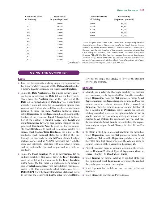
- Page 541 and 542: Supplementary Problems 511 publishe
- Page 543: Case 513 Frequency 7 6 5 4 3 2 1 0
- Page 547 and 548: Are You Going to Hate Your New Job?
- Page 549 and 550: 13.1 The Multiple Regression Model
- Page 551 and 552: 13.1 The Multiple Regression Model
- Page 553 and 554: Problems 523 Solution The following
- Page 555 and 556: 13.2 Significance Tests of the Regr
- Page 557 and 558: 13.2 Significance Tests of the Regr
- Page 559 and 560: Problems 529 13.9 Using the data in
- Page 561 and 562: 13.3 Residuals, Standard Error of t
- Page 563 and 564: 13.3 Residuals, Standard Error of t
- Page 565 and 566: 13.4 Interpreting Multiple Regressi
- Page 567 and 568: 13.4 Interpreting Multiple Regressi
- Page 569 and 570: Summary 539 SUMMARY OUTPUT Regressi
- Page 571 and 572: Supplementary Problems 541 TESTING
- Page 573 and 574: Case 543 ANALYZING THE DATABASES 1.
- Page 576 and 577: CHAPTER 14 Building Multiple Regres
- Page 578 and 579: 548 Chapter 14 Building Multiple Re
- Page 580 and 581: 550 Chapter 14 Building Multiple Re
- Page 582 and 583: 552 Chapter 14 Building Multiple Re
- Page 584 and 585: 554 Chapter 14 Building Multiple Re
- Page 586 and 587: 556 Chapter 14 Building Multiple Re
- Page 588 and 589: 558 Chapter 14 Building Multiple Re
- Page 590 and 591: 560 Chapter 14 Building Multiple Re
- Page 592 and 593: 562 Chapter 14 Building Multiple Re
- Page 594 and 595:
564 Chapter 14 Building Multiple Re
- Page 596 and 597:
566 Chapter 14 Building Multiple Re
- Page 598 and 599:
568 Chapter 14 Building Multiple Re
- Page 600 and 601:
570 Chapter 14 Building Multiple Re
- Page 602 and 603:
572 Chapter 14 Building Multiple Re
- Page 604 and 605:
574 Chapter 14 Building Multiple Re
- Page 606 and 607:
576 Chapter 14 Building Multiple Re
- Page 608 and 609:
578 Chapter 14 Building Multiple Re
- Page 610 and 611:
580 Chapter 14 Building Multiple Re
- Page 612 and 613:
582 Chapter 14 Building Multiple Re
- Page 614 and 615:
584 Chapter 14 Building Multiple Re
- Page 616 and 617:
586 Chapter 14 Building Multiple Re
- Page 618 and 619:
CHAPTER 15 Time-Series Forecasting
- Page 620 and 621:
590 Chapter 15 Time-Series Forecast
- Page 622 and 623:
592 Chapter 15 Time-Series Forecast
- Page 624 and 625:
594 Chapter 15 Time-Series Forecast
- Page 626 and 627:
596 Chapter 15 Time-Series Forecast
- Page 628 and 629:
598 Chapter 15 Time-Series Forecast
- Page 630 and 631:
600 Chapter 15 Time-Series Forecast
- Page 632 and 633:
602 Chapter 15 Time-Series Forecast
- Page 634 and 635:
604 Chapter 15 Time-Series Forecast
- Page 636 and 637:
606 Chapter 15 Time-Series Forecast
- Page 638 and 639:
608 Chapter 15 Time-Series Forecast
- Page 640 and 641:
610 Chapter 15 Time-Series Forecast
- Page 642 and 643:
612 Chapter 15 Time-Series Forecast
- Page 644 and 645:
614 Chapter 15 Time-Series Forecast
- Page 646 and 647:
616 Chapter 15 Time-Series Forecast
- Page 648 and 649:
618 Chapter 15 Time-Series Forecast
- Page 650 and 651:
620 Chapter 15 Time-Series Forecast
- Page 652 and 653:
622 Chapter 15 Time-Series Forecast
- Page 654 and 655:
624 Chapter 15 Time-Series Forecast
- Page 656 and 657:
626 Chapter 15 Time-Series Forecast
- Page 658 and 659:
628 Chapter 15 Time-Series Forecast
- Page 660 and 661:
630 Chapter 15 Time-Series Forecast
- Page 662 and 663:
632 Chapter 15 Time-Series Forecast
- Page 664 and 665:
634 Chapter 15 Time-Series Forecast
- Page 666 and 667:
636 Chapter 15 Time-Series Forecast
- Page 668 and 669:
638 Chapter 15 Time-Series Forecast
- Page 670 and 671:
640 Chapter 15 Time-Series Forecast
- Page 672 and 673:
642 Chapter 15 Time-Series Forecast
- Page 674 and 675:
CHAPTER 16 Analysis of Categorical
- Page 676 and 677:
646 Chapter 16 Analysis of Categori
- Page 678 and 679:
648 Chapter 16 Analysis of Categori
- Page 680 and 681:
650 Chapter 16 Analysis of Categori
- Page 682 and 683:
652 Chapter 16 Analysis of Categori
- Page 684 and 685:
654 Chapter 16 Analysis of Categori
- Page 686 and 687:
656 Chapter 16 Analysis of Categori
- Page 688 and 689:
658 Chapter 16 Analysis of Categori
- Page 690 and 691:
660 Chapter 16 Analysis of Categori
- Page 692 and 693:
662 Chapter 16 Analysis of Categori
- Page 694 and 695:
664 Chapter 16 Analysis of Categori
- Page 696 and 697:
666 Chapter 16 Analysis of Categori
- Page 698 and 699:
668 Chapter 16 Analysis of Categori
- Page 700 and 701:
CHAPTER 17 Nonparametric Statistics
- Page 702 and 703:
672 Chapter 17 Nonparametric Statis
- Page 704 and 705:
674 Chapter 17 Nonparametric Statis
- Page 706 and 707:
676 Chapter 17 Nonparametric Statis
- Page 708 and 709:
678 Chapter 17 Nonparametric Statis
- Page 710 and 711:
680 Chapter 17 Nonparametric Statis
- Page 712 and 713:
682 Chapter 17 Nonparametric Statis
- Page 714 and 715:
684 Chapter 17 Nonparametric Statis
- Page 716 and 717:
686 Chapter 17 Nonparametric Statis
- Page 718 and 719:
688 Chapter 17 Nonparametric Statis
- Page 720 and 721:
690 Chapter 17 Nonparametric Statis
- Page 722 and 723:
692 Chapter 17 Nonparametric Statis
- Page 724 and 725:
694 Chapter 17 Nonparametric Statis
- Page 726 and 727:
696 Chapter 17 Nonparametric Statis
- Page 728 and 729:
698 Chapter 17 Nonparametric Statis
- Page 730 and 731:
700 Chapter 17 Nonparametric Statis
- Page 732 and 733:
702 Chapter 17 Nonparametric Statis
- Page 734 and 735:
704 Chapter 17 Nonparametric Statis
- Page 736 and 737:
706 Chapter 17 Nonparametric Statis
- Page 738 and 739:
708 Chapter 17 Nonparametric Statis
- Page 740 and 741:
710 Chapter 17 Nonparametric Statis
- Page 742 and 743:
712 Chapter 17 Nonparametric Statis
- Page 744 and 745:
714 Chapter 17 Nonparametric Statis
- Page 746 and 747:
716 Chapter 17 Nonparametric Statis
- Page 748:
718 Chapter 17 Nonparametric Statis
- Page 751 and 752:
Italy’s Piaggio Makes a Comeback
- Page 753 and 754:
18.1 Introduction to Quality Contro
- Page 755 and 756:
18.1 Introduction to Quality Contro
- Page 757 and 758:
18.1 Introduction to Quality Contro
- Page 759 and 760:
18.1 Introduction to Quality Contro
- Page 761 and 762:
18.1 Introduction to Quality Contro
- Page 763 and 764:
18.2 Process Analysis 733 18.2 PROC
- Page 765 and 766:
18.2 Process Analysis 735 FIGURE 18
- Page 767 and 768:
18.2 Process Analysis 737 FIGURE 18
- Page 769 and 770:
18.3 Control Charts 739 charts are
- Page 771 and 772:
18.3 Control Charts 741 UCL and LCL
- Page 773 and 774:
18.3 Control Charts 743 Using the s
- Page 775 and 776:
18.3 Control Charts 745 Compute R R
- Page 777 and 778:
18.3 Control Charts 747 Sample n Ou
- Page 779 and 780:
18.3 Control Charts 749 In computin
- Page 781 and 782:
18.3 Control Charts 751 below the c
- Page 783 and 784:
Problems 753 18.6 A machine operato
- Page 785 and 786:
Problems 755 a. 125 X bar Chart 3.0
- Page 787 and 788:
Formulas 757 identifying the effect
- Page 789 and 790:
Supplementary Problems 759 five con
- Page 791 and 792:
Analyzing the Databases 761 12.5 X
- Page 793 and 794:
Using the Computer 763 Sample Mean
- Page 795 and 796:
APPENDIX A Tables Table A.1: Random
- Page 797 and 798:
Appendix A Tables 767 TABLE A.2 Bin
- Page 799 and 800:
Appendix A Tables 769 TABLE A.2 Bin
- Page 801 and 802:
Appendix A Tables 771 TABLE A.2 Bin
- Page 803 and 804:
Appendix A Tables 773 TABLE A.2 Bin
- Page 805 and 806:
Appendix A Tables 775 TABLE A.3 Poi
- Page 807 and 808:
Appendix A Tables 777 TABLE A.3 Poi
- Page 809 and 810:
Appendix A Tables 779 TABLE A.4 The
- Page 811 and 812:
Appendix A Tables 781 TABLE A.6 Cri
- Page 813 and 814:
Appendix A Tables 783 TABLE A.7 Per
- Page 815 and 816:
Appendix A Tables 785 TABLE A.7 Per
- Page 817 and 818:
Appendix A Tables 787 TABLE A.7 Per
- Page 819 and 820:
Appendix A Tables 789 TABLE A.7 Per
- Page 821 and 822:
Appendix A Tables 791 TABLE A.7 Per
- Page 823 and 824:
Appendix A Tables 793 TABLE A.9 Cri
- Page 825 and 826:
Appendix A Tables 795 TABLE A.10 Cr
- Page 827 and 828:
Appendix A Tables 797 n 2 n 1 = .02
- Page 829 and 830:
Appendix A Tables 799 TABLE A.13 p-
- Page 831 and 832:
Appendix A Tables 801 TABLE A.13 p-
- Page 833 and 834:
Appendix A Tables 803 TABLE A.14 Cr
- Page 835 and 836:
APPENDIX B Answers to Selected Odd-
- Page 837 and 838:
Appendix B Answers to Selected Odd-
- Page 839 and 840:
Appendix B Answers to Selected Odd-
- Page 841 and 842:
Appendix B Answers to Selected Odd-
- Page 843 and 844:
Appendix B Answers to Selected Odd-
- Page 845 and 846:
GLOSSARY A a posteriori After the e
- Page 847 and 848:
Glossary 817 decision table A matri
- Page 849 and 850:
Glossary 819 the statistic below th
- Page 851 and 852:
Glossary 821 ratio level data Highe
- Page 853:
Glossary 823 W weighted aggregate p
- Page 856 and 857:
826 Index Centerline. See also Cont
- Page 858 and 859:
828 Index DMAIC (Define, Measure, A
- Page 860 and 861:
830 Index Law of improbable events,
- Page 862 and 863:
832 Index Populations accessing for
- Page 864 and 865:
834 Index Samples defined, 5 depend
- Page 866:
836 Index grouped data versus, 17-1
- Page 869 and 870:
Decision Making at the CEO Level CE
- Page 871 and 872:
19.1 The Decision Table and Decisio
- Page 873 and 874:
19.2 Decision Making Under Uncertai
- Page 875 and 876:
19.2 Decision Making Under Uncertai
- Page 877 and 878:
19.2 Decision Making Under Uncertai
- Page 879 and 880:
Problems C19-13 d. Compute an oppor
- Page 881 and 882:
19.3 Decision Making Under Risk C19
- Page 883 and 884:
19.3 Decision Making Under Risk C19
- Page 885 and 886:
19.3 Decision Making Under Risk C19
- Page 887 and 888:
Problems C19-21 Much information ha
- Page 889 and 890:
19.4 Revising Probabilities in Ligh
- Page 891 and 892:
19.4 Revising Probabilities in Ligh
- Page 893 and 894:
19.4 Revising Probabilities in Ligh
- Page 895 and 896:
Problems C19-29 The worth of the sa
- Page 897 and 898:
Problems C19-31 Decision Making at
- Page 899 and 900:
Supplementary Problems C19-33 for e
- Page 901 and 902:
Supplementary Problems C19-35 Decis
- Page 903 and 904:
Case C19-37 Following these initiat
- Page 905 and 906:
Critical Values from the t Distribu