Analytic Solutions to a Family of Lotka-Volterra Related Differential ...

3.5
3.0
2.5
x 2.0 2
1.5
n = 3
n = 4
1.0
n = ∞
0.5
0.5 1.0 1.5 2.0 2.5 3.0 3.5
x 1
n = 2
(14)
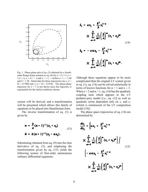
Fig. 1. Phase-plane plot of eq. (3) obtained by a fourthorder
Runge-Kutta solution to eq. (8) for n = 2 ( ), n =
3 ( ), n = 4 ( ) and n = 4 ( )when a = c = 1.00
and b = 1.30. Initial data for these trajectories are x 1 (t =
0) = 0.7000 and x 2 (t = 0) = 0.5556. The phase-plane
trajectory for n = 1 is not shown since the trajectory is
exponential for the initial conditions chosen.
system will be derived, and a transformation
will be presented which allows this family of
equations to be placed into Hamiltonian form.
The inverse transformation of eq. (3) is
given by
Although these equations appear to be more
complicated than the original LV system given
in eq. (1), eq. (14) can be solved analytically in
terms of known functions for " = 1 and n # 3.
When n = 2 and " = 1, eq. (14) has the quadratic
coupling term which appears in the LV
predator-prey model [i.e., eq. (1)] as well as
quadratic terms dependent only on x 1 and x 2
(which is reminiscent of the LV competition
model [18]).
The phase space trajectories of eq. (14) are
determined by
(13)
Substituting obtained from eq. (9) into the time
derivative of eq. (3), and employing the
transformation given by eq. (13) yields the
following system of first-order autonomous
ordinary differential equations:
(15)
6