Untitled - International Meteor Organization

168 WGN, the Journal of the IMO 38:5 (2010)
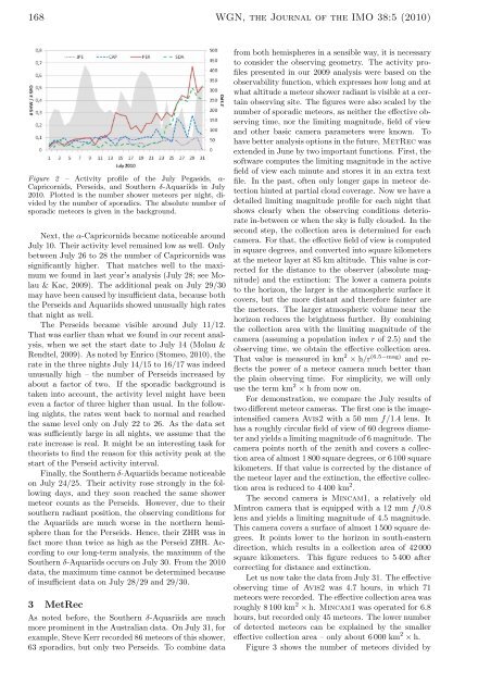
Figure 2 – Activity profile of the July Pegasids, α-
Capricornids, Perseids, and Southern δ-Aquariids in July
2010. Plotted is the number shower meteors per night, divided
by the number of sporadics. The absolute number of
sporadic meteors is given in the background.
Next, the α-Capricornids became noticeable around
July 10. Their activity level remained low as well. Only
between July 26 to 28 the number of Capricornids was
significantly higher. That matches well to the maximum
we found in last year’s analysis (July 28; see Molau
& Kac, 2009). The additional peak on July 29/30
may have been caused by insufficient data, because both
the Perseids and Aquariids showed unusually high rates
that night as well.
The Perseids became visible around July 11/12.
That was earlier than what we found in our recent analysis,
when we set the start date to July 14 (Molau &
Rendtel, 2009). As noted by Enrico (Stomeo, 2010), the
rate in the three nights July 14/15 to 16/17 was indeed
unusually high – the number of Perseids increased by
about a factor of two. If the sporadic background is
taken into account, the activity level might have been
even a factor of three higher than usual. In the following
nights, the rates went back to normal and reached
the same level only on July 22 to 26. As the data set
was sufficiently large in all nights, we assume that the
rate increase is real. It might be an interesting task for
theorists to find the reason for this activity peak at the
start of the Perseid activity interval.
Finally, the Southern δ-Aquariids became noticeable
on July 24/25. Their activity rose strongly in the following
days, and they soon reached the same shower
meteor counts as the Perseids. However, due to their
southern radiant position, the observing conditions for
the Aquariids are much worse in the northern hemisphere
than for the Perseids. Hence, their ZHR was in
fact more than twice as high as the Perseid ZHR. According
to our long-term analysis, the maximum of the
Southern δ-Aquariids occurs on July 30. From the 2010
data, the maximum time cannot be determined because
of insufficient data on July 28/29 and 29/30.
3 MetRec
As noted before, the Southern δ-Aquariids are much
more prominent in the Australian data. On July 31, for
example, Steve Kerr recorded 86 meteors of this shower,
63 sporadics, but only two Perseids. To combine data
from both hemispheres in a sensible way, it is necessary
to consider the observing geometry. The activity profiles
presented in our 2009 analysis were based on the
observability function, which expresses how long and at
what altitude a meteor shower radiant is visible at a certain
observing site. The figures were also scaled by the
number of sporadic meteors, as neither the effective observing
time, nor the limiting magnitude, field of view
and other basic camera parameters were known. To
have better analysis options in the future, MetRec was
extended in June by two important functions. First, the
software computes the limiting magnitude in the active
field of view each minute and stores it in an extra text
file. In the past, often only longer gaps in meteor detection
hinted at partial cloud coverage. Now we have a
detailed limiting magnitude profile for each night that
shows clearly when the observing conditions deteriorate
in-between or when the sky is fully clouded. In the
second step, the collection area is determined for each
camera. For that, the effective field of view is computed
in square degrees, and converted into square kilometers
at the meteor layer at 85 km altitude. This value is corrected
for the distance to the observer (absolute magnitude)
and the extinction: The lower a camera points
to the horizon, the larger is the atmospheric surface it
covers, but the more distant and therefore fainter are
the meteors. The larger atmospheric volume near the
horizon reduces the brightness further. By combining
the collection area with the limiting magnitude of the
camera (assuming a population index r of 2.5) and the
observing time, we obtain the effective collection area.
That value is measured in km 2 × h/r (6.5−mag) and reflects
the power of a meteor camera much better than
the plain observing time. For simplicity, we will only
use the term km 2 × h from now on.
For demonstration, we compare the July results of
two different meteor cameras. The first one is the imageintensified
camera Avis2 with a 50 mm f/1.4 lens. It
has a roughly circular field of view of 60 degrees diameter
and yields a limiting magnitude of 6 magnitude. The
camera points north of the zenith and covers a collection
area of almost 1 800 square degrees, or 6100 square
kilometers. If that value is corrected by the distance of
the meteor layer and the extinction, the effective collection
area is reduced to 4400 km 2 .
The second camera is Mincam1, a relatively old
Mintron camera that is equipped with a 12 mm f/0.8
lens and yields a limiting magnitude of 4.5 magnitude.
This camera covers a surface of almost 1500 square degrees.
It points lower to the horizon in south-eastern
direction, which results in a collection area of 42000
square kilometers. This figure reduces to 5400 after
correcting for distance and extinction.
Let us now take the data from July 31. The effective
observing time of Avis2 was 4.7 hours, in which 71
meteors were recorded. The effective collection area was
roughly 8 100 km 2 × h. Mincam1 was operated for 6.8
hours, but recorded only 45 meteors. The lower number
of detected meteors can be explained by the smaller
effective collection area – only about 6 000 km 2 × h.
Figure 3 shows the number of meteors divided by