Models of diffusion-limited uptake of trace elements in fossils and ...

Trace element uptake in fossils? 3761
ing DMD, faster diffusion rates have been documented for
some elements in the near surface (outer few nm) of calcite
crystals (Stipp et al., 1992). Because the bioapatite that
composes fossils is nanocrystalline, even after fossilization,
relatively fast intracrystalline diffusion may permit DMD.
Given sufficient time, all three models can explain homogeneous
compositions documented in some fossils, and all
three processes might occur simultaneously. The central
points of the following discussion are to demonstrate that
(1) the exact fossilization process is irrelevant to dating
problems, as long as boundaries were simple and trace element
uptake was limited by diffusion, and (2) appropriate
mathematical treatment of data simplifies interpretation
and error analysis.
3.2. Mathematic treatment
All solutions to the diffusion equation can be expressed
in terms of the dimensionless variables reduced time (t 0 ) and
reduced distance squared (X 02 ). For this paper, t 0 = D eff t/l 2
and X 0 = X/l, where D eff is the effective diffusion coefficient,
t is time, l is the half-width of the tissue considered, and X is
distance. Some workers prefer t 0 =[D eff t/l 2 ] 1/2 . The effective
diffusion coefficient (D eff ) is the ratio of the tracer diffusion
rate (D) in a fluid and the partition coefficient between biogenic
apatite and diagenetic or pedogenic fluids (K d ), corrected
for porosity (r) and tortuosity (s), i.e., D eff = Dr/
K d s 2 . Note that in applications discussed below D eff is a
measured value, so it automatically accounts for contributions
from porosity and tortuosity, and that K d , r, and s
are presumed constant, so solutions to the diffusion equation
scale equivalently with either D or D eff . If material diffuses
from a single (planar) boundary, e.g., from dentine
into enamel across the dentine–enamel interface, and/or
diffusion profiles are short (t 0 is small) then a semi-infinite
solution is used, and X 0 is expressed as the distance from
that surface or boundary (where X 0 = 0). In contrast, if
material diffuses between 2 parallel interfaces, e.g., inward
from both the interior and exterior surfaces of cortical
bone, then a plane sheet solution is used, and X 0 is expressed
as the distance from the midpoint between the
two boundaries: X 0 = 0 is the center of the sheet, and
X 0 =1, 1 are the boundaries.
Most models assume a fixed boundary condition, i.e.,
that the concentration at any bounding surface (C o ) is fixed
at time t = 0. The initial concentration of the diffusing species
(e.g., U, REE etc.) in the fossilizing tissue is also commonly
assumed to be zero, and although this assumption is
not required, it closely approximates biogenic compositions
(e.g., see Driessens and Verbeeck, 1990; Kohn et al., 1999).
Mathematically all models predict the change in trace element
concentration (C), or its normalized concentration,
(C 0 , where C 0 = C/C o ), as a function of reduced distance
(X 0 ) and reduced time (t 0 ). Solutions to the diffusion equation
were obtained from Crank (1975), specifically Eqs.
3.13 (semi-infinite medium solution for modeling short diffusion
profiles in enamel), either 2.54 or 2.68 (plane sheet
solutions for modeling long diffusion profiles in bone),
and 13.13 plus 13.18 (semi-infinite medium solution for
modeling DR).
In this discussion, the term t 0 Dep is used to describe the
time since initiation of the boundary condition and is equivalent
to the total duration, or t 0 , of a model. In practice,
t 0 Dep is proportional to the true depositional age, with a
proportionality constant of D eff /l 2 . The term t 0 app is used
to describe the apparent age at position X 0 within a sample.
In practice, t 0 app is proportional to the measured age with
the same proportionality constant, D eff /l 2 .
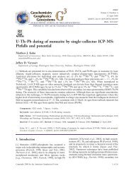
Examples for the DA plane sheet model show increases
in trace element concentration over time, with the rate of
increase dependent on distance from the boundaries and
time (Fig. 2A). These concentration profiles must be converted
to an age. For short diffusion profiles, e.g., REE in
enamel, this may be accomplished by fitting an inverse
C/Co
1.0
0.8
0.6
0.4
0.2
X’=0.9
X’=0.7
X’=0.5
X’=0.3
X’=0.1
t' app =
t' True
∫
[ C/C o ]dt'
t'=0
t' Dep
t'app
1.0
0.8
0.6
0.4
0.2
0.0
0.0
0.5
0.0 0.2 0.4 0.6 0.8 1.0 0.0 0.2 0.4 0.6 0.8 1.0
0.0 0.2 0.4 0.6 0.8 1.0
t' Dep t' Dep Edge Distance
X’=1.0
X’=0.9
X’=0.7
X’=0.5
X’=0.3
X’=0.1
Figure
2C
A B C
t'app
1.0
0.9
0.8
0.7
0.6
1-X'
1-X' 2
t' Dep = 1.0
Fig. 2. Numerical results of plane sheet DA model for U uptake over a range of timescales. (A) Concentration vs. time for different distances.
Boundary is at X 0 = 1, and has constant composition C o throughout. Apparent age is determined by integrating concentration curve (in terms
of C/C o ) at a particular value of X 0 over duration t 0 Dep , and ratioing to t0 Dep . (B) Apparent age ðt0 app Þ vs. depositional age ðt0 Dep
, or age of initial
establishment of fixed boundary condition). At boundary (X 0 = 1) apparent and depositional ages coincide, so the slope is 1. For long times,
the slope of t 0 app
for all positions approaches 1 as U is saturated. Circle shows integrated composition corresponding to gray region in Fig. 2A.
Box shows data points plotted in Fig. 2C. (C) t 0 app
vs. distance, showing quadratic form with respect to distance, and linearity with respect to
distance squared. Note that any function that is linear in X 02 is also linear in 1 X 02 .
Core