Be exposure age calculator MATLAB function reference Version 2

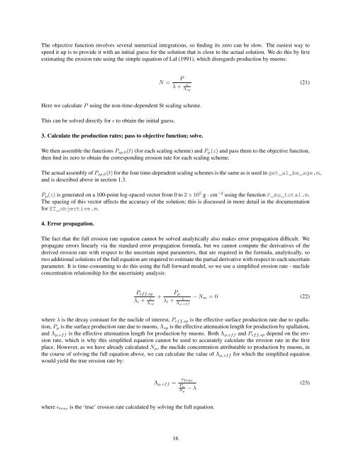
The objective function involves several numerical integrations, so finding its zero can be slow. The easiest way to
speed it up is to provide it with an initial guess for the solution that is close to the actual solution. We do this by first
estimating the erosion rate using the simple equation of Lal (1991), which disregards production by muons:
P
N =
λ +
ɛ
(21)
Λ sp
Here we calculate P using the non-time-dependent St scaling scheme.
This can be solved directly for ɛ to obtain the initial guess.
3. Calculate the production rates; pass to objective function; solve.
We then assemble the functions P sp,0 (t) (for each scaling scheme) and P µ (z) and pass them to the objective function,
then find its zero to obtain the corresponding erosion rate for each scaling scheme.
The actual assembly of P sp,0 (t) for the four time-dependent scaling schemes is the same as is used in get_al_be_age.m,
and is described above in section 1.3.
P µ (z) is generated on a 100-point log-spaced vector from 0 to 2 × 10 5 g · cm −2 using the function P_mu_total.m.
The spacing of this vector affects the accuracy of the solution; this is discussed in more detail in the documentation
for ET_objective.m.
4. Error propagation.
The fact that the full erosion rate equation cannot be solved analytically also makes error propagation difficult. We
propagate errors linearly via the standard error propagation formula, but we cannot compute the derivatives of the
derived erosion rate with respect to the uncertain input parameters, that are required in the formula, analytically, so
two additional solutions of the full equation are required to estimate the partial derivative with respect to each uncertain
parameter. It is time-consuming to do this using the full forward model, so we use a simplified erosion rate - nuclide
concentration relationship for the uncertainty analysis:
P eff,sp
ɛ +
Λ sp
λ i +
λ i +
P µ
ɛ − N m = 0 (22)
Λ µ,eff
where λ is the decay constant for the nuclide of interest, P eff,sp is the effective surface production rate due to spallation,
P µ is the surface production rate due to muons, Λ sp is the effective attenuation length for production by spallation,
and Λ µ,eff is the effective attenuation length for production by muons. Both Λ µ,eff and P eff,sp depend on the erosion
rate, which is why this simplified equation cannot be used to accurately calculate the erosion rate in the first
place. However, as we have already calculated N µ , the nuclide concentration attributable to production by muons, in
the course of solving the full equation above, we can calculate the value of Λ µ,eff for which the simplified equation
would yield the true erosion rate by:
Λ µ,eff =
ɛ true
P µ
N µ
− λ
(23)
where ɛ true is the ‘true’ erosion rate calculated by solving the full equation.
16