Linear Algebra Notes Chapter 9 MULTIPLE EIGENVALUES AND ...
Linear Algebra Notes Chapter 9 MULTIPLE EIGENVALUES AND ...
Linear Algebra Notes Chapter 9 MULTIPLE EIGENVALUES AND ...

Create successful ePaper yourself
Turn your PDF publications into a flip-book with our unique Google optimized e-Paper software.
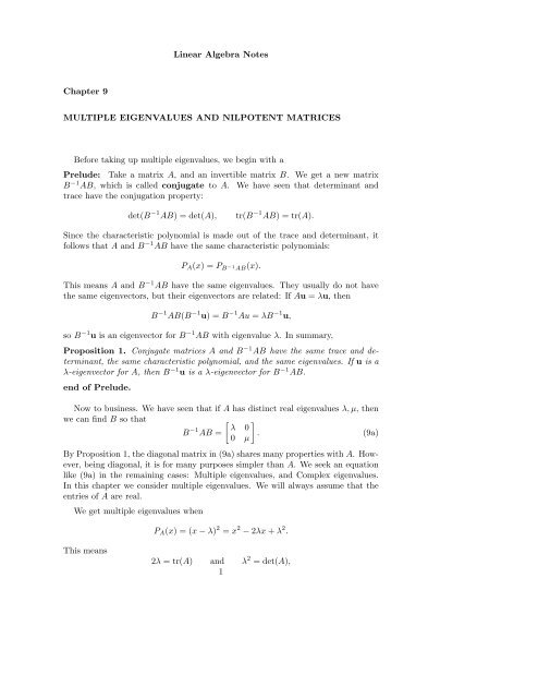
<strong>Linear</strong> <strong>Algebra</strong> <strong>Notes</strong><br />
<strong>Chapter</strong> 9<br />
<strong>MULTIPLE</strong> <strong>EIGENVALUES</strong> <strong>AND</strong> NILPOTENT MATRICES<br />
Before taking up multiple eigenvalues, we begin with a<br />
Prelude: Take a matrix A, and an invertible matrix B. We get a new matrix<br />
B −1 AB, which is called conjugate to A. We have seen that determinant and<br />
trace have the conjugation property:<br />
det(B −1 AB) = det(A),<br />
tr(B −1 AB) = tr(A).<br />
Since the characteristic polynomial is made out of the trace and determinant, it<br />
follows that A and B −1 AB have the same characteristic polynomials:<br />
P A (x) = P B −1 AB(x).<br />
This means A and B −1 AB have the same eigenvalues. They usually do not have<br />
the same eigenvectors, but their eigenvectors are related: If Au = λu, then<br />
B −1 AB(B −1 u) = B −1 Au = λB −1 u,<br />
so B −1 u is an eigenvector for B −1 AB with eigenvalue λ. In summary,<br />
Proposition 1. Conjugate matrices A and B −1 AB have the same trace and determinant,<br />
the same characteristic polynomial, and the same eigenvalues. If u is a<br />
λ-eigenvector for A, then B −1 u is a λ-eigenvector for B −1 AB.<br />
end of Prelude.<br />
Now to business. We have seen that if A has distinct real eigenvalues λ, µ, then<br />
we can find B so that<br />
[ ]<br />
B −1 λ 0<br />
AB = . (9a)<br />
0 µ<br />
By Proposition 1, the diagonal matrix in (9a) shares many properties with A. However,<br />
being diagonal, it is for many purposes simpler than A. We seek an equation<br />
like (9a) in the remaining cases: Multiple eigenvalues, and Complex eigenvalues.<br />
In this chapter we consider multiple eigenvalues. We will always assume that the<br />
entries of A are real.<br />
We get multiple eigenvalues when<br />
P A (x) = (x − λ) 2 = x 2 − 2λx + λ 2 .<br />
This means<br />
2λ = tr(A) and λ 2 = det(A),<br />
1
2<br />
so<br />
4 det(A) = [tr(A)] 2 (9b)<br />
The matrices with only one eigenvalue are those whose trace and determinant satisfy<br />
(9b). Note that λ = 1 2<br />
tr(A) will be real, since the entries of A are real.<br />
There are then two possibilities for A. Either A = λI, or A ≠ λI. Assume<br />
A ≠ λI. Then, in contrast to previous situations, we cannot conjugate A to a<br />
diagonal matrix. But we can do almost as well:<br />
Proposition 2. If A has only one eigenvalue λ, and A ≠ λI, then there is an<br />
invertible matrix B such that<br />
[ ]<br />
B −1 λ 1<br />
AB = .<br />
0 λ<br />
The difference from the distinct-eigenvalue case is the 1 in the upper right entry,<br />
which cannot be made zero, no matter how we choose B.<br />
Proof. We give a recipe for finding B. As before, first find a λ-eigenvector u, for<br />
A. Now take any vector v which is not proportional to u. Let B 1 be the matrix<br />
defined by<br />
B 1 e 1 = u, B 1 e 2 = v.<br />
We do a familiar computation<br />
So<br />
B −1<br />
1 AB 1e 1 = B1 −1 Au = λB−1 1 u = λe 1.<br />
[ ]<br />
B1 −1 λ g<br />
AB 1 = ,<br />
0 h<br />
for some numbers g, h that we don’t yet know. But in fact, h = λ. To see this,<br />
note that<br />
[ ]<br />
2λ = tr(A) = tr(B1 −1<br />
λ g<br />
AB 1) = tr = λ + h,<br />
0 h<br />
(we used Proposition 1 at the second equality) so indeed, λ = h. So we in fact have<br />
[ ]<br />
B1 −1 λ g<br />
AB 1 = .<br />
0 λ<br />
Now g ≠ 0, since if g = 0 we[ would]<br />
have A = λI, but we are assuming A ≠ λI.<br />
g 0<br />
Now conjugate further using , and get<br />
0 1<br />
[ ] [<br />
g<br />
−1<br />
0 λ g<br />
0 1 0 λ<br />
] [ ]<br />
g 0<br />
=<br />
0 1<br />
[ ]<br />
λ 1<br />
.<br />
0 λ<br />
This shows that if we take<br />
then<br />
[ ]<br />
g 0<br />
B = B 1 ,<br />
0 1<br />
B −1 AB =<br />
[ ]<br />
λ 1<br />
,<br />
0 λ
3<br />
as claimed in Proposition 2.<br />
□<br />
so<br />
Now if you want to compute A n , you could first note that<br />
A n = (B<br />
[ ] n [ ]<br />
λ 1 λ<br />
n<br />
nλ<br />
=<br />
n−1<br />
0 λ 0 λ n<br />
[ ]<br />
[ ]<br />
λ 1<br />
B −1 ) n λ<br />
n<br />
nλ<br />
= B<br />
n−1<br />
0 λ<br />
0 λ n B −1 .<br />
(9b)<br />
(9c)<br />
Actually, there is a much better formula for A n , but first let’s have an example to<br />
illustrate what we’ve seen so far.<br />
Example:<br />
A =<br />
[ ]<br />
0 4<br />
.<br />
−1 4<br />
We find P A (x) = (x − 2) 2 so λ = 2 is a multiple eigenvalue of A. Our formula for<br />
eigenvectors gives (b, λ − a) = (4, 2). Scaling, we can take the eigenvector to be<br />
u = (2, 1). Now we choose any another vector v which is not proportional to u.<br />
Let us take v = e 1 , so we have<br />
B 1 =<br />
[ ]<br />
2 1<br />
.<br />
1 0<br />
We then compute<br />
[ ]<br />
B1 −1 0 1<br />
= ,<br />
1 −2<br />
and<br />
[<br />
B1 −1 0 1<br />
AB 1 =<br />
1 −2<br />
] [<br />
0 4<br />
−1 4<br />
] [ ]<br />
2 1<br />
=<br />
1 0<br />
[ ]<br />
2 −1<br />
.<br />
0 2<br />
So g = −1 and we take<br />
[ ]<br />
−1 0<br />
B = B 1 =<br />
0 1<br />
[ ]<br />
−2 1<br />
.<br />
−1 0<br />
To check our calculations we compute<br />
[<br />
−2<br />
]<br />
1<br />
−1 0<br />
B −1 AB =<br />
[ ]<br />
2 1<br />
.<br />
0 2<br />
So B = does the job, as predicted by Proposition 2.<br />
[ ] n<br />
2 1<br />
Continuing further using equation (9c), we have =<br />
0 2<br />
A n = B<br />
[ ] [ ]<br />
2<br />
n<br />
n2 n−1<br />
0 2 n B −1 2<br />
=<br />
n − n2 n n2 n+1<br />
−n2 n−1 2 n + n2 n .<br />
[ ]<br />
2<br />
n<br />
n2 n−1<br />
0 2 n , so
4<br />
We could write this as a sum<br />
[ ] [ ]<br />
A n 2<br />
n<br />
0<br />
=<br />
0 2 n + n2 n−1 −2 4<br />
.<br />
−1 2<br />
The first matrix in this sum is the diagonal matrix whose diagonal entries are the<br />
powers of the eigenvalue of A. The second matrix (considered without the factor<br />
n2 n−1 ), is almost A, but with the eigenvalue 2 subtracted from the diagonal entries<br />
of A. Let us call this matrix A 0 . So<br />
A 0 =<br />
[<br />
−2<br />
]<br />
4<br />
−1 2<br />
Thus, we could write our formula for A n as<br />
=<br />
[ ]<br />
0 − 2 4<br />
= A − 2I.<br />
−1 4 − 2<br />
A n = 2 n I + n2 n−1 A 0 .<br />
This is a formula is much simpler than (9c), and it holds in general.<br />
[ ]<br />
a b<br />
Proposition 3. Let A = be a matrix with P<br />
c d<br />
A = (x − λ) 2 . Define the new<br />
matrix<br />
[ ]<br />
a − λ b<br />
A 0 =<br />
.<br />
c d − λ<br />
[ ]<br />
0 0<br />
Then A 2 0 = , and<br />
0 0<br />
A n = λ n I + nλ n−1 A 0 .<br />
The point of Proposition 3 is that it allows us to compute A n in a much easier<br />
way than equation (9c). We don’t have to find B to use Proposition [ 3. ] However,<br />
0 0<br />
we will use B to prove Proposition 3. The key point is that A 2 0 = .<br />
0 0<br />
Proof. We use our earlier formula<br />
from Proposition 2. Note that<br />
A = B<br />
[ ]<br />
λ 1<br />
B −1 ,<br />
0 λ<br />
[ ]<br />
λ 1<br />
= λI +<br />
0 λ<br />
[ ]<br />
0 1<br />
,<br />
0 0<br />
so<br />
A = B<br />
[ ]<br />
λ 1<br />
B −1 = B(λI +<br />
0 λ<br />
[ ]<br />
0 1<br />
)B −1 = B(λI)B −1 + B<br />
0 0<br />
[ ]<br />
0 1<br />
B −1 .<br />
0 0<br />
Since λI commutes with every matrix, we have B(λI)B −1 = λI, so<br />
A = λI + B<br />
[ ]<br />
0 1<br />
B −1 .<br />
0 0
5<br />
But also A = λI + A 0 , so<br />
λI + A 0 = A = λI + B<br />
Subtracting λI from both sides, we get<br />
[ ]<br />
0 1<br />
A 0 = B B −1 .<br />
0 0<br />
Hence<br />
because<br />
[ ] 2<br />
0 1<br />
=<br />
0 0<br />
[ ]<br />
A 2 0 1<br />
0 = B B −1 B<br />
0 0<br />
[ ] 2<br />
0 1<br />
= B B −1<br />
0 0<br />
[ ]<br />
0 0<br />
= B B −1<br />
0 0<br />
=<br />
[<br />
0 0<br />
0 0<br />
]<br />
,<br />
[ ]<br />
0 1<br />
B −1 .<br />
0 0<br />
[ ]<br />
0 1<br />
B −1<br />
0 0<br />
[ ]<br />
0 0<br />
. That was the key point. Now we have<br />
0 0<br />
A n = (λI + A 0 ) n .<br />
Inside the parentheses, we have two matrices. One of them, λI, commutes with all<br />
matrices, and the other one, A 0 , squares to zero.<br />
Now let us pause, and temporarily empty our minds of all thoughts of A and A 0 .<br />
Clear the table. On this empty table, we put two matrices [ X, ] Y with the following<br />
0 0<br />
two properties. First, XY = Y X, and second, Y 2 = . Now we add them<br />
0 0<br />
and raise to powers. The second power is<br />
(X + Y ) 2 = (X + Y )(X + Y ) = XX + XY + Y X + Y Y = X 2 + 2XY,<br />
because XY = Y X and Y 2 = 0. In the general power<br />
(X + Y ) n = (X + Y )(X + Y ) · · · (X + Y )<br />
we get each term by choosing either X or Y in each factor. Since they commute,<br />
we can put the Y ’s together, which will give zero unless we have at most one power<br />
of Y . So we either choose X in each factor (one such term), or we choose Y in one<br />
factor and X in all the others (n such terms). Thus<br />
(X + Y ) n = X n + nX n−1 Y.<br />
Now we resurrect A and A 0 , and finish our calculation: Since (λI) n = λ n I, we<br />
get<br />
A n = (λI + A 0 ) n = λ n I + nλ n−1 A 0 ,
6<br />
as claimed.<br />
□<br />
A matrix is called nilpotent if some power of it is zero. It turns out, for 2 × 2<br />
matrices Y as we are considering here, that if Y n = 0, then already Y 2 = 0 (see<br />
exercise 9.4). So a 2×2 matrix is nilpotent if either it is already zero, or if it squares<br />
to zero.<br />
We may summarize the main points in this chapter as follows. Any matrix A with<br />
a multiple eigenvalue λ is a scalar matrix λI plus a nilpotent matrix A 0 = A − λI.<br />
If [ A is]<br />
not itself a scalar matrix, [ then]<br />
A 0 ≠ 0. In that case A is conjugate to<br />
λ 1<br />
0 1<br />
, and A<br />
0 λ<br />
0 is conjugate to . This last matrix does not involve λ. In<br />
0 0<br />
particular, all matrices A with multiple [ eigenvalues ] have their nilpotent parts A 0<br />
0 1<br />
being conjugate to the same matrix .<br />
0 0<br />
Exercise 9.1. For each of the[ following ] matrices A, find the eigenvalue λ, and a<br />
λ 1<br />
matrix B such that B −1 AB = .<br />
0 λ<br />
[ ]<br />
6 1<br />
(a) A =<br />
[<br />
−1 8<br />
]<br />
1 −1<br />
(b) A =<br />
[<br />
1 −1<br />
]<br />
1 0<br />
(c) A =<br />
[<br />
1 1<br />
]<br />
0 1<br />
(d) A =<br />
−1 2<br />
(To make life easier for the grader, please choose v = e 1 in each problem. Your<br />
B’s will all be the same, having 1 in the upper right corner.)<br />
[ ]<br />
λ 1<br />
Exercise 9.2. Show that every eigenvector of is proportional to e<br />
0 λ<br />
1 . (Hint:<br />
Just calculate.)<br />
Exercise 9.3. Let A be a matrix with multiple eigenvalue λ, and let u be an eigenvector<br />
of A. Assume that A is not a scalar matrix. Prove the following statements.<br />
(a) Every eigenvector of A is proportional to u. (Hint: Proposition 1.)<br />
(b) A 0 u = (0, 0)<br />
(c) If v is a vector for which A 0 v = (0, 0), then v is an eigenvector of A.<br />
(Taken together, these facts mean that A has exactly one eigenline, which consists<br />
precisely of the vectors sent to (0, 0) by A 0 . )<br />
[ ]<br />
0 0<br />
Exercise 9.4. Suppose A n = for some n ≥ 0.<br />
0 0<br />
(a) What are the eigenvalues of A? (Hint: Apply A repeatedly to both sides of<br />
the equation Au = λu. )<br />
(b) Compute A 2 . (Hint: Use Proposition 3, and the value of λ from part (a). )<br />
Exercise 9.5. Suppose λ = 0 is the only eigenvalue of A. Does this imply that A<br />
is nilpotent?
7<br />
Exercise 9.6. Show that the nilpotent matrices are precisely those of the form<br />
[ ]<br />
a b<br />
A =<br />
c −a<br />
with a 2 + bc = 0.<br />
(You have to show two things: First, that every nilpotent matrix has this form.<br />
Second, that every matrix of this form is nilpotent.)