Introduction to Probability, by Dimitri P ... - satrajit mukherjee

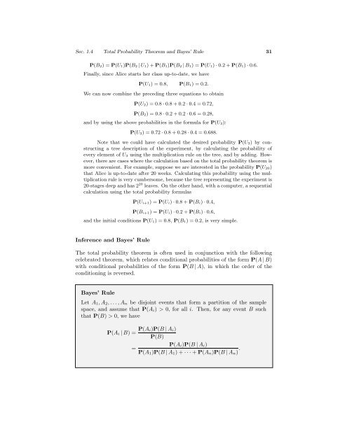
Sec. 1.4 Total Probability Theorem and Bayes’ Rule 31
P(B 2)=P(U 1)P(B 2 | U 1)+P(B 1)P(B 2 | B 1)=P(U 1) · 0.2+P(B 1) · 0.6.
Finally, since Alice starts her class up-to-date, we have
P(U 1)=0.8, P(B 1)=0.2.
We can now combine the preceding three equations to obtain
P(U 2)=0.8 · 0.8+0.2 · 0.4 =0.72,
P(B 2)=0.8 · 0.2+0.2 · 0.6 =0.28,
and by using the above probabilities in the formula for P(U 3):
P(U 3)=0.72 · 0.8+0.28 · 0.4 =0.688.
Note that we could have calculated the desired probability P(U 3)byconstructing
a tree description of the experiment, by calculating the probability of
every element of U 3 using the multiplication rule on the tree, and by adding. However,
there are cases where the calculation based on the total probability theorem is
more convenient. For example, suppose we are interested in the probability P(U 20)
that Alice is up-to-date after 20 weeks. Calculating this probability using the multiplication
rule is very cumbersome, because the tree representing the experiment is
20-stages deep and has 2 20 leaves. On the other hand, with a computer, a sequential
calculation using the total probability formulas
P(U i+1) =P(U i) · 0.8+P(B i) · 0.4,
P(B i+1) =P(U i) · 0.2+P(B i) · 0.6,
and the initial conditions P(U 1)=0.8, P(B 1)=0.2, is very simple.
Inference and Bayes’ Rule
The total probability theorem is often used in conjunction with the following
celebrated theorem, which relates conditional probabilities of the form P(A | B)
with conditional probabilities of the form P(B | A), in which the order of the
conditioning is reversed.
Bayes’ Rule
Let A 1 ,A 2 ,...,A n be disjoint events that form a partition of the sample
space, and assume that P(A i ) > 0, for all i. Then, for any event B such
that P(B) > 0, we have
P(A i | B) = P(A i)P(B | A i )
P(B)
P(A i )P(B | A i )
=
P(A 1 )P(B | A 1 )+···+ P(A n )P(B | A n ) .