Building Models from Experimental Data. - elkintonlab

More documents

Recommendations

Info

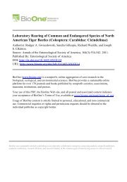
Pathogen-Driven Outbreaks Revisited 113 Figure 5: Cycle periodicity and the parameter range that permits stable cycles for the short-epidemic model. The cycle period and the chance of unstable cycles both increase as fecundity l decreases. of stable cycles given the high levels of heterogeneity in susceptibility in the data. Given that our transmission data do not preclude the possibility of outbreaks, we also compare the model to gypsy moth population data more quantitatively. Specifically, gypsy moth populations typically fluctuate over about four orders of magnitude in density (Elkinton and Liebhold 1990), and so we ask, Does the model show this amplitude of fluctuations for realistic parameter values We define amplitude to mean the difference in density between peaks and troughs of the population cycle. Figure 5 shows that cycle period increases with increasing values of pathogen carryover f and decreasing values of fecundity l and heterogeneity in susceptibility C, matching the effects of these parameters on the boundary between limit cycles and a stable equilibrium. Figure 5 also shows that the model can match the observed 9-yr period of gypsy moth population fluctuations for a broad range of parameter values. The further requirement of an amplitude of fluctuation of about four orders of magnitude, however, means that fecundity l must be about 5 (not shown). Here, “fecundity” is interpreted to mean “net population change in the near-absence of the disease” rather than “eggs per egg mass” (Hassell et al. 1976). Under this definition, observed net gypsy moth fecundity l is about 11 (Elkinton et al. 1996). Given that the variance in net gypsy moth fecundity from year to year is large ( SE=9.1, n= 8), model and data are in approximate agreement. More quantitatively, in figure 6, we show the best fit of the model to a time series for gypsy moth (Ostfeld et al. 1996). By first transforming the data according to log e[N t1/N t] (Turchin and Taylor 1992), we were able to fit the nondimensionalized short-epidemic model to the data using only fecundity l, heterogeneity C, and pathogen survival f (app. A; note that we assume g =0). We found the best-fit values of these parameters by calculating the sum of the squared differences between the model and the data for parameter combinations that spanned the area of parameter space in which the model shows stable cycles. To generate the figure, we then used the model output for the best-fit values of the parameters and varied the ratio ¯n/m until we had achieved a good fit between the host density predicted by the model and the host density in the data (app. A), as determined again by least squares. Although this time series is short and is based on a sampling area of only 0.16 ha (in particular the low points of each cycle are based on very small sample sizes; Ostfeld et al. 1997), nevertheless, figure 6 demonstrates that the model does a good job of reproducing the data. Also, estimates Figure 6: Best fit of the short-epidemic model to time series data for gypsy moth Lymantria dispar (Ostfeld et al. 1996). Parameter values are fecundity l = 5.5, heterogeneity in susceptibility C=0.86, and pathogen overwinter survival f =15. Table 1 gives the value of n¯ .
114 The American Naturalist of mean transmission ¯n and heterogeneity C from these data are close to the parameters estimated both from our experimental data and from single epidemics (table 1). Discussion Our work has led us to a general conclusion that is identical to that of Anderson and May’s (1981) work, that host-pathogen interactions are likely to cause outbreaks in forest-insect populations. Our models include realistic features of insect-pathogen interactions that are missing from Anderson and May’s models, however, and this additional realism leads us to different conclusions about which biological details are important in driving outbreaks. Specifically, Anderson and May emphasized the importance of high pathogen survival in causing long-period cycles, but our models have shown instead that cycles are possible even with relatively low pathogen survival because of the high average susceptibility of early stage larvae relative to later-stage larvae. Also, Anderson and May used continuous-generation host-pathogen models; because the simplest such models give stable population dynamics, a major thrust of their work was that the long-lived infectious stage, typical of insect pathogens, destabilizes their models enough to give long-period cycles. In contrast, because our models realistically assume discrete host generations, they are likely to show unstable dynamics. Consequently, we instead emphasize a mechanism that stabilizes what would otherwise be unstable cycles, specifically, host heterogeneity in susceptibility. In this respect, discrete-generation host-pathogen models are more like discrete-generation host-parasitoid models (Hassell et al. 1991), a point first made by Briggs and Godfray (1996). The differences between our conclusions and those of Anderson and May are due to differences in model structure for which our gypsy moth data provide strong support. First, our experimental data strongly support the inclusion of host heterogeneity in susceptibility and delays between infection and death in our epidemic model equations (1) and (2) (Dwyer et al. 1997). Second, discrete host generations are an obvious feature of gypsy moth populations, and the experiments of Murray and Elkinton (1989, 1990) have made clear the importance of virus contamination of egg masses for the initiation of epidemics. Breaking the gypsy moth life cycle into epidemic and interepidemic periods is therefore a crucial feature of our model. This structure is further supported by the ability of the models to accurately describe the dynamics of gypsy moth populations at spatial scales of entire regions and over timescales of decades (figs. 5, 6). In particular, our estimates of the average transmission rate ¯n and of host heterogeneity in susceptibility C from long-term data are similar to estimates from short-term experiments (table 1). Comparison of our model to the model of Briggs and Godfray (1996) suggests that host heterogeneity in susceptibility is an especially important detail. Briggs and Godfray’s main model is similar to ours in allowing for discrete host generations and a single epidemic each year. A major difference, however, is that instead of explicitly incorporating a distribution of host heterogeneity in susceptibility, they incorporate a kind of phenomenological heterogeneity in transmission, following a formulation used in host-parasitoid models. In the resulting model, cycles are only found for a very narrow range of parameters, unless long-term pathogen survival is allowed. Our model most closely matches Briggs and Godfray’s main model if we set single-generation pathogen carryover f ≤ 1 and long-term pathogen survival g =0. For these parameter values, however, our model produces cycles for a broad range of values of fecundity l and host heterogeneity C. Even when Briggs and Godfray allowed for longterm pathogen survival ( g 1 0), the period of the cycles apparently never exceeded four generations. These differences suggest that host heterogeneity in susceptibility is of profound importance for the dynamics of insect-pathogen interactions and that the details of how heterogeneity is incorporated matter a great deal. For the particular case of host heterogeneity in susceptibility, our results suggest that a mechanistic approach is crucial. Our data, however, suggest some caveats. First, the short-epidemic model shows that the levels of heterogeneity in susceptibility that we observe in our data are likely to stabilize what might otherwise be unstable cycles, but the confidence intervals on our data are large enough that the importance of heterogeneity in susceptibility in leading to stable cycles is an open question. In particular, Bonsall et al. (1999) showed that adding nondisease direct density dependence to Briggs and Godfray’s (1996) host-pathogen model also tends to stabilize unstable cycles. Because this direct density dependence is typical of gypsy moth populations at high density (Carter et al. 1991), the work of Bonsall et al. (1999) suggests that both host heterogeneity and competition for food act to stabilize disease-driven fluctuations in gypsy moth populations. In fact, there is at least a short list of other biological details of gypsy moth population dynamics that are missing from our model but that are known to be important in gypsy moth population dynamics. Indeed, low-density gypsy moth populations may be kept in check by density-dependent small-mammal predation (Elkinton and Liebhold 1990). Evidence for such density dependence is equivocal (Elkinton et al. 1996), but evidence for the importance of small-mammal predation on late instars and pupae, especially by the white-footed mouse Peromyscus leucopus, is strong. Changes in low-
Page 1 and 2: Pathogen‐Driven Outbreaks in Fore
Page 3 and 4: 106 The American Naturalist D’Ami
Page 5 and 6: 108 The American Naturalist Figure
Page 7 and 8: 110 The American Naturalist such th
Page 9: 112 The American Naturalist Table 1
Page 13 and 14: 116 The American Naturalist differe
Page 15 and 16: 118 The American Naturalist APPENDI
Page 17: 120 The American Naturalist phenolo

Building Models from Experimental Data. - elkintonlab

Create successful ePaper yourself

Delete template?

Save as template?