MATLAB Functions for Mie Scattering and Absorption

5
E
E
s!
s"
ikr
e
= cos"
# S2(cos!
)
$ ikr
ikr
e
= sin"
# S1(cos!
)
ikr
with the scattering amplitudes S 1 and S 2
S (cos%
) =
1
S (cos%
) =
2
"
!
n=
1
"
!
n=
1
2n
+ 1
( an#
n
n(
n + 1)
2n
+ 1
( an$
n
n(
n + 1)
+ b $ );
n
+ b # )
n
n
n
(p.111)
(4.74)
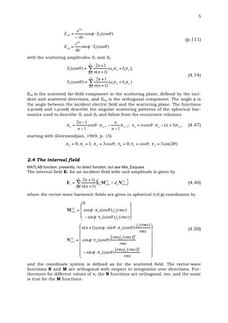
E s θ is the scattered far-field component in the scattering plane, defined by the incident
and scattered directions, and E s φ is the orthogonal component. The angle φ is
the angle between the incident electric field and the scattering plane. The functions
π n(cosθ) and τ n(cosθ) describe the angular scattering patterns of the spherical harmonics
used to describe S 1 and S 2 and follow from the recurrence relations
2n
! 1
n
#
n
= cos$
"#
n! 1
! #
n!
2;
%
n
= ncos$
"#
n
! ( n + 1)
#
n!
1
(4.47)
n ! 1
n ! 1
starting with (Deirmendjian, 1969, p. 15)
#
0
= 0;
#
1
= 1; #
2
= 3cos!
; "
0
= 0; "
1
= cos!
; "
2
= 3cos(2!
)
2.4 The internal field
MATLAB function: presently, no direct function, but see Mie_Esquare
The internal field E 1 for an incident field with unit amplitude is given by
! "
n=
1
(1)
(1)
( c n
M # d N )
2n
+ 1)
E
1
=
o1n
n e1n
(4.40)
n(
n + 1)
where the vector-wave harmonic fields are given in spherical (r,θ,φ) coordinates by
M
N
(1)
o1n
(1)
e1n
& 0
#
$
!
= $ cos+
'*
n(cos)
jn(
rmx)
!
$
!
% ( sin+
',
n(cos)
jn(
rmx)
"
&
jn(
rmx)
#
$ n(
n + 1)cos+
' sin)
'*
n(cos)
!
$
rmx !
$
[ rmxj rmx !
n(
)]'
= $ cos+
',
n(cos)
!
$
rmx
!
$
[ rmxjn(
rmx)]'
!
( sin+
'*
n(cos)
%
rmx "
(4.50)
and the coordinate system is defined as for the scattered field. The vector-wave
functions N and M are orthogonal with respect to integration over directions. Furthermore
for different values of n, the N functions are orthogonal, too, and the same
is true for the M functions.