Ocean Circulation - Water Types and Water Masses

1556 OCEAN CIRCULATION / Water Types and Water Masses 

Water Types and Water Masses 

W J Emery, University of Colorado, Boulder, CO, USA 

Copyright 2003 Elsevier Science Ltd. All Rights Reserved. 

problems, there is very little research directed at 

improving our knowledge of water mass distributions 

and their changes over time. 

Introduction 

Much of what is known today about the currents of the 

deep ocean has been inferred from studies of the water 

properties such as temperature, salinity, dissolved 

oxygen, and nutrients. These are quantities that can be 

observed with standard hydrographic measurement 

techniques which collect temperatures and samples of 

water with a number of sampling bottles strung along 

a wire to provide the depth resolution needed. Salinity 

or ‘salt content’ is then measured by an analysis of the 

water sample, which combined with the corresponding 

temperature value at that ‘bottle’ sample yields 

temperature and salinity as a function of depth of the 

sample. Modern observational methods have in part 

replaced this sample bottle method with electronic 

profiling systems, at least for temperature and salinity, 

but many of the important descriptive quantities such 

as oxygen and nutrients still require bottle samples 

accomplished today with a ‘rosette’sampler integrated 

with the electronic profiling systems. These new 

electronic profiling systems have been in use for over 

30 years, but still the majority of data useful for 

studying the properties of the deep and open ocean 

come from the time before the advent of modern 

electronic profiling system. This knowledge is important 

in the interpretation of the data since the 

measurements from sampling bottles have very different 

error characteristics than those from modern 

electronic profiling systems. 

This article reviews the mean properties of the open 

ocean, concentrating on the distributions of the major 

water masses and their relationships to the currents of 

the ocean. Most of this information is taken from 

published material, including the few papers that 

directly address water mass structure, along with the 

many atlases that seek to describe the distribution of 

water masses in the ocean. Coincident with the shift 

from bottle sampling to electronic profiling is the shift 

from publishing information about water masses and 

ocean currents in large atlases to the more routine 

research paper. In these papers the water mass characteristics 

are generally only a small portion, requiring 

the interested descriptive oceanographer to go to 

considerable trouble to extract the information he or 

she may be interested in. While water mass distributions 

play a role in many of today’s oceanographic 

What is a Water Mass 

The concept of a ‘water mass’ is borrowed from 

meteorology, which classifies different atmospheric 

characteristics as ‘air masses’. In the early part of the 

twentieth century physical oceanographers also 

sought to borrow another meteorological concept 

separating the ocean waters into ‘warm’ and ‘cold’ 

water spheres. This designation has not survived in 

modern physical oceanography but the more general 

concept of water masses persists. Some oceanographers 

regard these as real, objective physical entities, 

building blocks from which the oceanic stratification 

(vertical structure) is constructed. At the opposite 

extreme, other oceanographers consider water masses 

to be mainly descriptive words, summary shorthand 

for pointing to prominent features in property distributions. 

The concept adopted for this discussion is squarely 

in the middle, identifying some ‘core’ water mass 

properties that are the building blocks. In most parts of 

the ocean the stratification is defined by mixing in both 

vertical and horizontal orientations of the various 

water masses that advect into the location. Thus, in the 

maps of the various water mass distributions a 

‘formation region’ is identified where it is believed 

that the core water mass has acquired its basic 

characteristics at the surface of the ocean. This 

introduces a fundamental concept first discussed by 

Iselin (1939), who suggested that the properties of the 

various subsurface water masses were originally 

formed at the surface in the source region of that 

particular water mass. Since temperature and salinity 

are considered to be ‘conservative properties’ (property 

is only changed at the sea surface), these characteristics 

would slowly erode as the water properties 

were advected at depth to various parts of the ocean. 

Descriptive Tools: The TS Curve 

Before focusing on the global distribution of water 

masses, it is appropriate to introduce some of the basic 

tools used to describe these masses. One of the most 

basic tools is the use of property versus property 

plots to summarize an analysis by making extrema 

easy to locate. The most popular of these is the

OCEAN CIRCULATION / Water Types and Water Masses 1557 

temperature–salinity or TS diagram, which relates 

density to the observed values of temperature and 

salinity. Originally the TS curve was constructed for a 

single hydrographic cast and thus related the TS values 

collected for a single bottle sample with the salinity 

computed from that sample. In this way there was a 

direct relationship between the TS pair and the depth 

of the sample. As the historical hydrographic record 

expanded it became possible to compute TS curves 

from a combination of various temperature–salinity 

profiles. This approach amounted to plotting the TS 

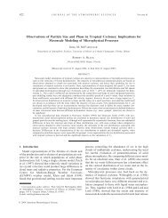
curve as a scatter diagram (Figure 1) where the salinity 

values were then averaged over a selected temperature 

interval to generate a discrete TS curve. The TS curve 

shown in Figure 1, which is an average of all of the 

data in a 101 square just north east of Hawaii, 

shows features typical of those that can be found 

in all TS curves. As it turned out the temperature– 

salinity pair remained the same while the depth of this 

pair oscillated vertically by tens of meters, resulting in 

the absence of a precise relationship between TS pairs 

and depth. As sensed either by ‘bottle casts’ or by 

electronic profilers, these vertical variations express 

themselves as increased variability in the temperature 

or salinity profiles while the TS curve continues to 

retain its shape, now independent of depth. Hence a 

composite TS curve computed from a number of 

closely spaced hydrographic stations no longer has a 

Salinity, ‰ 

32 33 34 35 36 37 

30 

25 

∆ S,T 

600 

m 

100 

Tropical 

upper 

20 

500 

150 

Tropical 

Sal. Max. 

Temperature (°C) 

15 

400 

200 

N. Pacific 

central 

10 

300 

500 

N. Pacific 

Intermediate 

and AAIW 

(mixing) 

5 

1000 

N. Pacific 

10−20°N 

150−160°W 

Deep 

0 

200 

100 

5000 

0 

T/S pairs = 9428 

Figure 1 Example of TS ‘scatter plot’ for all data within a 101square with mean TS curve (center line) and curves for one standard 

deviation in salinity on either side.


specific relationship between temperature, salinity 

and depth. 

As with the more traditional ‘single station’ TS 

curve, these area average TS curves can be used to 

define and locate water masses. This is done by 

locating extrema in salinity associated with particular 

water masses. The salinity minimum in the TS curve of 

Figure 1 is at about 101C, where there is a clear 

divergence of TS values as they move up the temperature 

scale from the coldest temperatures near the 

bottom of the diagram. There are two separate clusters 

of points at this salinity minimum temperature with 

one terminating at about 131C and the other transitioning 

on up to the warmest temperatures. It is this 

termination of points that results in a sharp turn in the 

mean TS curve and causes a very wide standard 

deviation. These two clusters of points represent two 

different intermediate level water masses. The relatively 

high salinity values that appear to terminate at 

131C represent the Antarctic Intermediate Water 

(AIW) formed near the Antarctic continent, reaching 

its northern terminus after flowing up from the 

south. The coincident less salty points indicate the 

presence of North Pacific Intermediate Water moving 

south from its formation region in the northern Gulf of 

Alaska. 

While there is no accepted practice in water mass 

terminology, it is generally accepted that a ‘water type’ 

refers to a single point on a characteristic diagram such 

as a TS curve. As introduced above, ‘water mass’ refers 

to some portion or segment of the characteristic curve, 

which describes the ‘core properties’ of that water 

mass. In the above example the salinity characteristics 

of the two intermediate waters were salinity minima, 

which were the overall characteristic of the two 

intermediate waters. We note that the extrema associated 

with a particular water mass may not remain at 

the same salinity value. Instead, as one moves away 

from the formation zone for the AIW, which is at the 

oceanographic ‘polar front’, the sharp minimum that 

marks the AIW water which has sunk from the surface 

down to about 1000 m starts to erode, broadening the 

salinity minimum and slowly increasing its magnitude. 

By comparing conditions of the salinity extreme at a 

location with salinity characteristics typical of the 

formation region one can estimate the amount of the 

source water mass that is still present at the distant 

location. Called the ‘core-layer’ method, this procedure 

was a crucial development in the early study of 

the ocean water masses and long-term mean currents. 

Many variants of the TS curve have been introduced 

over the years. One particularly instructive form was a 

‘volumetric TS curve’. Here the oceanographer subjectively 

decides just how much volume is associated 

with a particular water mass. This becomes a threedimensional 

relationship, which can then be plotted in 

a perspective format (Figure 2). In this plot the two 

horizontal axes are the usual temperature and salinity, 

while the elevation represents the volumes with those 

particular TS characteristics. For this presentation, 

only the deeper water mass characteristics have been 

plotted, which can be seen by the restriction of the 

temperature scale to 1.01C to 4.01C. Arrows have 

been added to show just which parts of the ocean 

various features have come from. That the Atlantic is 

the saltiest of the oceans is very clear with a branch to 

high salinity values at higher temperatures. The most 

voluminous water mass is the Pacific Deep Water that 

fills most of the Pacific below the intermediate waters 

at about 1000 m. 

Global Water Mass Distribution 

Before turning to the TS curve description of the water 

masses, it is necessary to indicate the geographic 

distribution of the basic water masses. The reader is 

cautioned that this article only treats the major water 

masses, which most oceanographers accept and agree 

upon. If a particular region is of interest close 

inspection will reveal a great variety of smaller water 

mass classifications; these can be almost infinite, as 

higher resolution is obtained in both horizontal and 

vertical coverage. 

Table 1 presents the TS characteristics of the world’s 

water masses. In the table are listed the area name, the 

corresponding acronym, and the appropriate temperature 

and salinity range. Recall that the property 

extreme erodes moving away from the source region, 

so it is necessary to define a range of properties. This is 

also consistent with the view that a water mass refers 

to a segment of the TS curve rather than a single point. 

As is traditionally the case, the water masses have 

been divided into deep and abyssal waters, intermediate 

waters, and upper waters. While the upper 

waters have the largest property ranges, physically 

they occupy the least amount of ocean volume. The 

reverse is true of the deep and bottom waters, which 

have a fairly restricted range but occupy a substantial 

portion of the ocean. Since most ocean water mass 

properties are established at the ocean’s surface, those 

water masses which spend most of their time isolated 

far from the surface will erode the least and have the 

longest lifetime. Surface waters, on the other hand, are 

strongly influenced by fluctuations at the ocean 

surface, which rapidly erodes the water mass properties. 

In mean TS curves, as in Figure 1, the spread 

of the standard deviation at the highest temperatures 

reflect this influence from the heat and fresh water 

flux exchange that occurs near and at the ocean’s 

surface.


World ocean 

Pacific 

Pacific deep 

4° 

34.40 

Atlantic 

0° 

1° 

2° 

Potential temperature (°C) 

3° 

34.50 34.70 34.80 34.90 35.00 

2° 

3° 

4° 

34.40 

1° 

34.50 34.60 34.70 34.80 34.90 35.00 

0° 

Salinity (‰) 

Southern 

Indian 

Figure 2 

Simulated three-dimensional T–S–V diagram for the cold water masses of the World Ocean. 

Accompanying the table are global maps of water 

masses at all three of these levels. The upper waters in 

Figure 3 have the most complex distribution with 

significant meridional and zonal changes. A ‘best 

guess’ at the formation regions for the corresponding 

water mass is indicated by the hatched regions. For its 

relatively small size, the Indian Ocean has a very 

complex upper water mass structure. This is caused by 

some unique geographic conditions. First is the monsoon, 

which completely changes the wind patterns 

twice a year. This causes reversals in ocean currents, 

which also influence the water masses by altering the 

contributions of the very saline Arabian Gulf and the 

fresh Bay of Bengal into the main body of the Indian 

Ocean. All of the major rivers in India flow to the east 

and discharge into the Bay of Bengal, making it a very 

fresh body of ocean water. To the west of the Indian 

subcontinent is the Arabian Sea with its connection to 

the Persian Gulf and the Red Sea, both locations of 

extremely salty water, making the west side of India 

very salty and the east side very fresh. The other upper 

ocean water masses in the Indian Ocean are those 

associated with the Antarctic Circumpolar Current 

(ACC), which are found at all of the longitudes in the 

Southern Ocean. 

As the largest ocean basin, the Pacific has the 

strongest east–west variations in upper water masses, 

with east and west central waters in both the north and 

south hemispheres. Unique to the Pacific is the fairly 

wide band of the Pacific Equatorial Water, which is 

strongly linked to the equatorial upwelling, which 

may not exist in El Niño years. None of the other two 

ocean basins have this equatorial water mass in the 

upper ocean. The Atlantic has northern hemisphere 

upper water masses that can be separated east–west 

while the South Atlantic upper water mass cannot be 

separated east–west into two parts. Note the interaction 

between the North Atlantic and the Arctic Ocean 

through the Norwegian Sea and Fram Strait. Also in 

these locations are found the source regions for a 

number of Atlantic water masses. Compared with the 

other two oceans, the Atlantic has the most water mass 

source regions, which produce a large part of the deep 

and bottom waters of the world ocean. 

The chart of intermediate water masses in Figure 4 is 

much simpler than was the upper ocean water masses 

in Figure 3. This reflects the fact that there are far fewer 

intermediate waters and those that are present fill large 

volumes of the intermediate depth ocean. The North 

Atlantic has the most complex horizontal structure of


Table 1 

Temperature–salinity characteristics of the world’s water masses 

Layer Atlantic Ocean Indian Ocean Pacific Ocean 

Upper waters 

(0–500 m) 

Atlantic Subarctic Upper Water 

(ASUW) (0.0–4.01C, 

34.0–35.0%) 

Western North Atlantic Central 

Water (WNACW) (7.0–20.01C, 

35.0–36.7%) 

Eastern North Atlantic Central 

Water (ENACW) (8.0–18.01C, 

35.2–36.7%) 

South Atlantic Central Water 

(SACW) (5.0–18.01C, 

34.3–35.8%) 

Bengal Bay Water (BBW) 

(25.0–291C, 28.0–35.0%) 

Arabian Sea Water (ASW) 

(24.0–30.01C, 35.5–36.8%) 

Indian Equatorial Water (IEW) 

(8.0–23.01C, 34.6–35.0%) 

Indonesian Upper Water (IUW) 

(8.0–23.01C, 34.4–35.0%) 

South Indian Central Water 

(SICW) (8.0–25.01C, 34.6– 

35.8%) 

Pacific Subarctic Upper Water 

(PSUW) (3.0–15.01C, 

32.6–33.6%) 

Western North Pacific Central 

Water (WNPCW) (10.0–22.01C, 

34.2–35.2%) 

Eastern North Pacific Central 

Water (ENPCW) (12.0–20.01C, 

34.2–35.0%) 

Eastern North Pacific Transition 

Water (ENPTW) (11.0–20.01C, 

33.8–34.3%) 

Pacific Equatorial Water (PEW) 

(7.0–23.01C, 34.5–36.0%) 

Western South Pacific Central 

Water (WSPCW) (6.0–22.01C, 

34.5–35.8%) 

Eastern South Pacific Central 

Water (ESPCW) (8.0–24.01C, 

34.4–36.4%) 

Eastern South Pacific Transition 

Water (ESPTW) (14.0–20.01C, 

34.6–35.2%) 

Intermediate waters 

(500–1500 m) 

Western Atlantic Subarctic 

Intermediate Water (WASIW) 

(3.0–9.01C, 34.0–35.1%) 

Eastern Atlantic Subarctic 

Intermediate Water (EASIW) 

(3.0–9.01C, 34.4–35.3%) 

Antarctic Intermediate Water 

(AAIW) (2–61C, 33.8–34.8%) 

Mediterranean Water (MW) 

(2.6–11.01C, 35.0–36.2%) 

Arctic Intermediate Water (AIW) 

( 1.5–3.01C, 34.7–34.9%) 


(AAIW) (2–101C, 33.8–34.8%) 

Indonesian Intermediate Water 

(IIW) (3.5–5.51C, 34.6– 

34.7%) 

Red Sea–Persian Gulf 

Intermediate Water (RSPGIW) 

(5–141C, 34.8–35.4%) 

Pacific Subarctic Intermediate 

Water (PSIW) (5.0–12.01C, 

33.8–34.3%) 

California Intermediate Water 

(CIW) (10.0–12.01C, 

33.9–34.4%) 

Eastern South Pacific Intermediate 

Water (ESPIW) (10.0–12.01C, 

34.0–34.4%) 


(AAIW) (2–101C, 33.8–34.5%) 

Deep and abyssal 

waters 

(1500 m-bottom) 

North Atlantic Deep Water 

(NADW) (1.5–4.01C, 

34.8–35.0%) 

Antarctic Bottom Water (AABW) 

( 0.9–1.71C, 34.64–34.72%) 

Arctic Bottom Water (ABW) 

( 1.8 to 10.51C, 34.88– 

34.94%) 

Circumpolar Deep Water (CDW) 

(1.0–2.01C, 34.62–34.73%) 

Circumpolar Surface Waters 

Circumpolar Deep Water (CDW) 

(0.1–2.01C, 34.62–34.73%) 

Subantarctic Surface Water 

(SASW) (3.2–15.01C, 

34.0–35.5%) 

Antarctic Surface Water (AASW) 

( 1.0–1.01C, 34.0–34.6%) 

the three oceans. Here intermediate waters form at the 

source regions in the northern North Atlantic. One 

exception is the Mediterranean Intermediate Water, 

which is a consequence of climatic conditions in the 

Mediterranean Sea. This salty water flows out through 

the Straits of Gibraltar at about 320 m depth, where it 

then descends to at least 1000 m, and maybe a bit 

more. It now sinks below the vertical range of the less 

saline Antarctic Intermediate Water (AAIW), instead 

joining with the higher salinity of the deeper North 

Atlantic Deep Water (NADW), which maintains the 

salinity maximum indicative of the NADW. 

In the Southern Ocean the formation region for the 

AAIW is marked as the location of the oceanic Polar

180° 

E 30°60°90° E E 120°150°150°120° W W 90°60°30°0°30° E 

Ice 

ASUW 

60° 

40° 

20° 

N 

0° 

S 

20° 

40° 

60° 

ASW 

Arab. Sea 

Water 

IEW 

Indian Equatorial Wat. 

S. Indian Centr. Water 

Bengal 

Bay 

Wat. 

Indo. Upper Wat. 

SICW 

BBW 


Antarctic Surface Water 

IUW 

WNPCW 

West. N. Pacific 

Centr. Water 

PEW 

P S U W 

Pac. Subarctic Upper Wa 

West. S. Pacific 


WSPCW 

E 30°60°90°120°150° E E 150°180°150°120°90°60° W W 60°30°0°30° E 

t. 

ENPCW 

East. N. Pacific 


Pacific Equatorial Water 

ESPCW 


Antarctic Surface Water 

East. N. Pacific 

Transition Water 

East. S. Pacific 


East. S. Pacific 

Transition Wat. 

Upper Waters 

(0−500m) 

WNACW 

West. N. Atl. 


ENACW 

East. N. Atl 

SACW 

. 

Centr. Wat. 

South Atlantic 



Antarctic Surface Wat. 

Figure 3 Global distribution of upper waters (0–500 m). Water masses are in abbreviated form with their boundaries indicated by solid lines. Formation regions for these water masses are 

marked by cross-hatching and labelled with the corresponding acronym title. 

A 

tl. 

U pper 

Wat. 

Subarctic 

60° 

40° 

20° 

N 

0° 

S 

20° 

40° 

60° 

OCEAN CIRCULATION / Water Types and Water Masses 1561

60° 

40° 

20° 

N 

0° 

S 

20° 

40° 

180° 

E 30°60°90° E E 120°150°150°120° W W 90°60°30°0°30° E 

Red Sea− 

Pers. Gulf 

Int. Water 

Antarctic Int. Water 

Indo. Int. Water 

IIW 

PSIW 

Pacific Subarctic Int. Water 

Calif. Int. Water 


CIW 

East S. Pacific 

Int. Wat. 

ESPI W 

WA SIW 

West. Atl. Subarctic 

Int. Water 

AIW 

EASIW 

East. Atl. 

M e d. 

Subarctic Int. Wat. 

W ater 


Arctic Int. Water 

MW 

MW 

60° 

40° 

20° 

N 

0° 

S 

20° 

40° 


60° 

AAIW 

AAIW 

Intermediate Waters 

(500 − 1500 m) 

AAIW 

60° 

E 30°60°90°120°150° E E 150°180°150°120°90°60° W W 60°30°0°30° E 

Figure 4 Global distribution of intermediate water (550–1500 m). Lines, labels and hatching follow the same format as described for Figure 3.


Front, which is known to vary considerably in strength 

and location, moving the formation region north and 

south. That this AAIW fills a large part of the ocean 

can be clearly seen in all of the ocean basins. In the 

Pacific the AAIWextends north to about 201 N, where 

it meets the NPIWas already noted from Figure 1. The 

AAIW reaches about the same latitude in the North 

Atlantic but it only reaches to about 51 S in the Indian 

Ocean. In the Pacific the northern intermediate waters 

are mostly from the North Pacific where the NPIW is 

formed. There is, however, another smaller volume 

intermediate water that is formed in the transition 

region west of California, mostly as a consequence of 

coastal upwelling. A similar intermediate water formation 

zone can be found in the south Pacific mainly 

off the coast of South America, which generates a 

minor intermediate water mass. 

The deep and bottom waters mapped in Figure 5 are 

restricted in their movements to the deeper reaches of 

the ocean. For this reason the 4000 m depth contour 

has been plotted in Figure 5 and a good correspondence 

can be seen between the distribution of bottom 

water and the deepest bottom topography. Some 

interesting aspects of this bottom water can be seen 

in the eastern South Atlantic. As the dense bottom 

water makes its way north from the Southern Ocean, 

in the east it runs into the Walvis Ridge, which blocks it 

from further northward extension. Instead the bottom 

water flows north along the west of the mid-Atlantic 

ridge and, finding a deep passage in the Romanche 

Gap, flows eastward and then south to fill the basin 

north of the Walvis Ridge. A similar complex pattern 

of distribution can be seen in the Indian Ocean, where 

the east and west portions of the basin fill from the 

south separately because of the central ridge in the 

bottom topography. In spite of the requisite depth of 

the North Pacific, the Antarctic Bottom Water 

(AABW) does not extend as far northward in the 

North Pacific. This means that some variant of the 

AABW, created by mixing with other deep and 

intermediate waters, occupies the most northern 

reaches of the deep North Pacific. Because the North 

Pacific is essentially ‘cut-off’ from the Arctic, there is 

no formation region of deep and bottom water in the 

North Pacific. 

The 3D TS curve of Figure 2 indicated that the most 

abundant water, mass marked by the highest peak in 

this TS curve, corresponded to Pacific Deep Water. In 

Table 1 there is listed something called ‘Circumpolar 

Deep Water’ in the deeper reaches of both the Pacific 

and Indian Oceans. This water mass is not formed at 

the surface but is instead a mixture of NADW, AABW, 

and the two intermediate waters present in the Pacific. 

The Antarctic Bottom Water (AABW) forms in the 

Weddell Sea as the product of very cold, dense, fresh 

water flowing off the continental shelf. It then sinks 

and encounters the upwelling NADW, which adds a 

bit of salinity to the cold, fresh water, making it even 

denser. This very dense product of Weddell Sea shelf 

water and NADW becomes the AABW, which then 

sinks to the very bottom and flows out of the Weddell 

Sea to fill most of the bottom layers of the world ocean. 

It is probable that a similar process works in the Ross 

Sea and some other areas of the continental shelf to 

form additional AABW, but the Weddell Sea is thought 

to be the primary formation region of AABW. 

Summary TS Relationships 

As pointed out earlier, one of the best ways to detect 

specific water masses is with the TS relationship, 

whether computed for single hydrographic casts or 

from an historical accumulation of such hydro casts. 

Here traditional practice is followed and the summary 

TS curves are divided into the major ocean basins 

starting with the Atlantic (Figure 6). Once again, the 

higher salinities typical of the Atlantic can be clearly 

seen. The highest salinities are introduced by the 

Mediterranean outflow marked as MW in Figure 6. 

This joins with water from the North Atlantic to 

become part of the NADW, which is marked by a 

salinity maximum in these TS curves. The AAIW is 

indicated by the sharp salinity minimum at lower 

temperatures. The source water for the AAIW is 

marked by a dark square in the figure. The AABW is a 

single point, which now does not represent a ‘water 

type’ but rather a water mass. The difference is that 

this water mass has very constant TS properties 

represented by a single point in the TS curves. Note 

that this is the densest water on this TS diagram (the 

density lines are shown as the dashed curves in the TS 

diagram marked with the value of s). 

The rather long segments stretching to the upper 

temperature and salinity values represent the upper 

waters in the Atlantic. While this occupies a large 

portion of the TS space, it only covers a relatively small 

part of the upper ocean when compared to the large 

volumes occupied by the deep and bottom water 

masses. From this TS diagram it can be seen that the 

upper waters are slightly different in the South 

Atlantic, the East North Atlantic and the West North 

Atlantic. Of these differences the South Atlantic differs 

more strongly from the other two than they do from 

each other. 

By comparison with Figure 6, the Pacific TS curves 

of the Pacific (Figure 7) are very fresh, with all but the 

highest upper water mass having salinities below 

35%. The bottom property anchoring this curve is the 

Circumpolar Deep Water (CDW), which is used to

60° 

40° 

20° 

N 

0° 

S 

20° 

Arctic 

Deep Water 

180° 

E 30°60°90° E E 120°150°150°120° W W 90°60°30°0°30° E 

ADW 

ADW 

Arctic 

Deep Water 

NADW 

ADW 

Arctic Deep Water 

60° 

40° 

20° 

N 

0° 

S 

20° 


40° 

Antarctic Bottom Water 

40° 

60° 


4000 m Depth contour 

Deep and Abyssal 

Waters 

(1500 m − bottom) 


AABW 

60° 

E 30°60°90°120°150° E E 150°180°150°120°90°60° W W 60°30°0°30° E 

Figure 5 Global distribution of deep and abyssal waters (1500–bottom). Contour lines describe the spreading of abyssal water (primarily AABW). The formation of NADW is indicated again by 

hatching and its spreading terminus, near the Antarctic, by a dashed line which also suggests the global communication of this deep water around the Antarctic.


20 

15 

SACW 

σ t = 26 

27 

WNACW 

ENACW 

MW 


10 

5 

28 

0 

−2 

AAIW 

NADW 

EASIW 

WASIW 

Atlantic Ocean 

AABW 

34 35 36 


Figure 6 Characteristic temperature–salinity (TS) curves for the main water masses of the Atlantic Ocean. Water masses are labelled 

by the appropriate acronym and core water properties are indicated by a dark square with an arrow to suggest their spread. The cross 

isopycnal nature of some of these arrows is not intended to suggest a mixing process but merely to connect source waters with their 

corresponding characteristic extrema. 

identify a wide range of TS properties that are known 

to be deep and bottom water but which have not been 

identified in terms of a specific formation region and 

TS properties. As with the AABW, a single point at the 

bottom of the curves represents the CDW. The 

relationship between the AAIW and the PSIW can be 

clearly seen in this diagram. The AAIW is colder and 

saltier than is the PSIW, which is generally a bit higher 

in the water column, indicated by the lower density of 

this feature. There are no external sources of deep 


20 

15 

10 

5 

PSIW 

ENPTW 

ESPCW 

ENPCW 

WNACW 

ESPTW 

PEW 

WSPCW 

σ = 26 

27 

28 

0 

−2 

AAIW 

CDW 

Pacific Ocean 

34 35 36 


Figure 7 

Characteristic TS curves for the main water masses of the Pacific Ocean.


salinity like with the Mediterranean Water in the 

Atlantic. Instead there is a confusing plethora of upper 

water masses that clearly separate the east–west and 

north–south portions of the basin. So we have Eastern 

North Pacific Central Water (ENPCW) and Western 

North Pacific Central Water (WNPCW), as well as 

Eastern South Pacific Central Water (ESPCW) and 

Western South Pacific Central Water (WSPCW). 

The central waters all refer to open ocean upper 

water masses. The more coastal water masses such as 

the Eastern North Pacific Transition Water (ENPTW) 

are typical of the change in upper water mass 

properties that occurs near the coastal regions. The 

same is true of the South Pacific as well. In general the 

fresher upper-layer water masses of the Pacific are 

located in the east where river runoff introduces a lot 

of fresh water into the upper ocean. To the west the 

upper water masses are saltier as shown by the 

quasilinear portions of the TS curves corresponding 

to the western upper water masses. The Pacific 

Equatorial Water (PEW) is unique in the Pacific 

probably due to well-developed equatorial circulation 

system. As seen in Figure 7, the PEW TS properties lie 

between the east and west central waters. 

The Indian Ocean TS curves in Figure 8 are quite 

different from either the Atlantic or the Pacific. 

Overall the Indian Ocean is quite a bit saltier than 

the Pacific but not quite as salty as the Atlantic. Also 

like the Atlantic, the Indian Ocean receives salinity 

input from a marginal sea as the Red Sea deposits its 

salt-laden water into the Arabian Sea. Its presence is 

noted in Figure 8 as the black box marked RSPGIW for 

the Red Sea–Persian Gulf Intermediate Water. Added 

at the sill depth of the Red Sea, this intermediate water 

contributes to a salinity maximum that is seasonally 

dependent. 

The bottom water is the same CDW that we saw in 

the Pacific. Unlike the Pacific, the Indian Ocean 

equatorial water masses are nearly isohaline above 

the point representing the CDW. In fact the line that 

represents the Indian Ocean Equatorial Water (IEW) 

runs almost straight up from the CDW at about 0.01C 

to the maximum temperature at 201C. There is 

expression of the AAIW in the curve that corresponds 

to the South Indian Ocean Central Water (SICW). A 

competing Indonesian Intermediate Water (IIW) has 

higher temperature and higher salinity characteristics 

which result in it having an only slightly lower density, 

creating the weak salinity minimum in the curve 

transitioning to the Indian Ocean Upper Water (IUW). 

The warmest and saltiest part of these TS curves 

represents the Arabian Sea Water (ASW) on the 

western side of the Indian subcontinent. 

Discussion and Conclusion 

The descriptions provided in this article cover only the 

most general of water masses, their core properties and 

their geographic distribution. In most regions of the 

ocean it is possible to resolve the water mass structure 

into even finer elements describing more precisely the 

differences in temperature and salinity. In addition, 

20 

BBW 

IEW 

σ = 26 

ASW 

15 

SICW 

27 


10 

IIW 

IUW 

RSPGIW 

28 

5 

AAIW 

0 

−2 

Indian Ocean 

CDW 

34 35 36 


Figure 8 Characteristic TS curves for the main water masses of the Indian Ocean. All lables as in Figure 6.

OPERATIONAL METEOROLOGY 1567 

other important properties can be used to specify 

water masses not obvious in TS space. While dissolved 

oxygen is often used to define water mass boundaries, 

care must be taken as this nonconservative property is 

influenced by biological activity and the chemical 

dissolution of dead organic material falling through 

the water column. Nutrients also suffer from modification 

within the water column, making their interpretation 

as water mass boundaries more difficult. 

Characteristic diagrams that plot oxygen against 

salinity or nutrients can be used to seek extrema that 

mark the boundaries of various water masses. 

The higher vertical resolution property profiles 

possible with electronic profiling instruments also 

make it possible to resolve water mass structure that 

was not even visible with the lower vertical resolution 

of earlier bottle sampling. Again, this complexity is 

only merited in local water mass descriptions and 

cannot be used on the global-scale description. At this 

global scale the descriptive data available from the 

accumulation of historical hydrographic data are 

adequate to map the large-scale water mass distribution, 

as has been done in this article. 

See also 

Boundary Layers: Ocean Mixed Layer. Convection: 

Convection in the Ocean. Coupled Ocean–Atmosphere 

Models. Ocean Circulation: General Processes; Surface–Wind 

Driven Circulation; Thermohaline Circulation. 

Further Reading 

Emery WJ and Meincke J (1986) Global water 

masses: summary and review. Oceanologica Acta 9: 

383–391. 

Mamayev OI (1975) Temperature–Salinity Analysis of 

World Ocean Waters. Elsevier Oceanography Series, 

#11, Elsevier Scientific Pub. Co., Amsterdam, 374 pp. 

Iselin CO’D (1939) The influence of vertical and lateral 

turbulence on the characteristics of the waters at middepths. 

Transactions of the American Geophysical Union 

20: 414–417. 

Pickard GL and Emery WJ (1992) Descriptive Physical 

Oceanography, 5th edn. Oxford, England: Pergamon 

Press. 

Reid JL (1973) Northwest Pacific Ocean Water in Winter. 

The Johns Hopkins Oceanographic Studies #5, Johns 

Hopkins Press, 96 pp. 

Sverdrup HU, Johnson MW and Fleming RH (1941) The 

Oceans. Prentice-Hall Inc., 1087 pp. 

Worthington LV (1976) On the North Atlantic Circulation. 

The Johns Hopkins Oceanographic Studies #6, Johns 

Hopkins Press, 110 pp. 

Worthington LV (1981) The water masses of the world 

ocean: some results of a fine-scale census. In: Warren BA 

and Wunsch C (eds) Evolution of Physical Oceanography, 

Ch. 2, pp. 42–69. Cambridge, MA: MIT Press. 

OPERATIONAL METEOROLOGY 

J V Cortinas Jr, University of Oklahoma/Cooperative 

Institute for Mesoscale Meteorological Studies, Norman, 

OK, USA 

W Blier, National Weather Service WASC, Monterey, 

CA, USA 

Copyright 2003 Elsevier Science Ltd. All Rights Reserved. 

Introduction 

Operational meteorology involves the generation and 

widespread dissemination of weather information. 

Although the types of weather-related information 

generated and the methods of distribution have 

evolved throughout the history of operational forecasting, 

the basic focus of this subdiscipline of the 

atmospheric sciences has remained unchanged: to use 

scientific knowledge about how the atmosphere 

behaves to develop and distribute useful forecasts of 

weather conditions. In its modern application, this 

process typically involves the acquisition, examination, 

and interpretation of vast quantities of both 

observational meteorological data and numerical 

forecast model output, and thus tends to be extremely 

computer intensive. The content of the disseminated 

weather products varies according to the issuing 

organization and the type of weather information 

required by its customers; typically, they include 

periodic reports and forecasts of weather conditions 

over particular geographic regions and notification of 

any anticipated or observed hazardous weather conditions. 

These products are disseminated in many 

ways, including dedicated electronic communications 

systems maintained by national and local governments, 

the World Wide Web, newspapers, radio, and 

television. 

Prior to the 1990s, countries with significant 

weather service programs generally relied on their 

respective national governments to provide weather 

information. While this practice is still common in

Ocean Circulation - Water Types and Water Masses

Create successful ePaper yourself

Delete template?

Save as template?