Binomial distribution - the Australian Mathematical Sciences Institute

A guide for teachers – Years 11 and 12 • {17}
want Pr(X ≥ 1) ≥ 0.9, since we only need to observe the species in one quadrat to know
that it is present in the forest. We have
Pr(X ≥ 1) ≥ 0.9 ⇐⇒ Pr(X = 0) ≤ 0.1
⇐⇒ (1 − k) n ≤ 0.1
⇐⇒ n ≥ log e (0.1)
log e (1 − k) .
For example: if k = 0.1, we need n ≥ 22; if k = 0.05, we need n ≥ 45; if k = 0.01, we need
n ≥ 230.
Exercise 4
a
p 0.01 0.05 0.2 0.35 0.5 0.65 0.8 0.95 0.99
µ X 0.2 1 4 7 10 13 16 19 19.8
sd(X ) 0.445 0.975 1.789 2.133 2.236 2.133 1.789 0.975 0.445
b
The standard deviation is smallest when |p−0.5| is largest; in this set of distributions,
when p = 0.01 and p = 0.99. The standard deviation is largest when p = 0.5.
Exercise 5
a
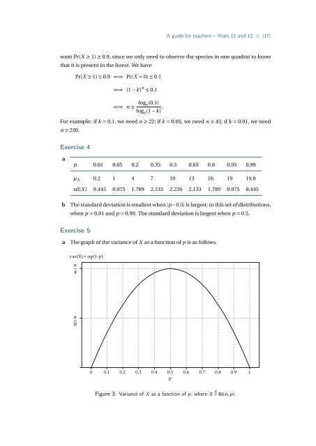
The graph of the variance of X as a function of p is as follows.
var(X) = np(1‐p)
4
8
0
0.1
0.2
0.3
0.4
0.5
p
0.6
0.7
0.8
0.9
1
Figure 3: Variance of X as a function of p, where X d = Bi(n, p).