THEOREM ON COMMUTATION IN THE PRINCIPAL PART

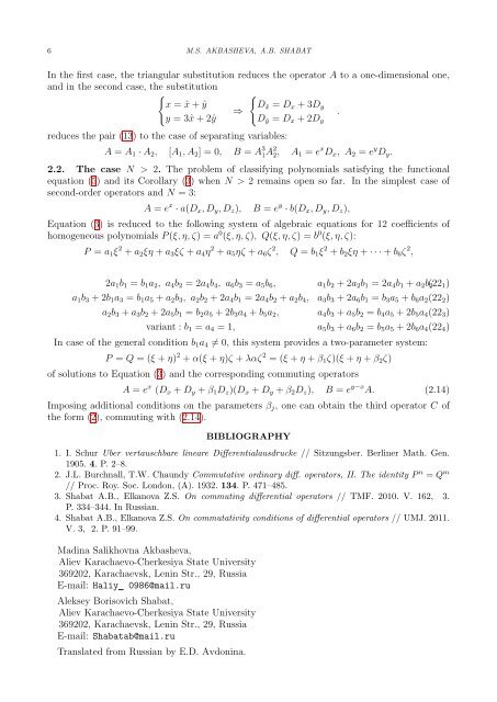
6 M.S. AKBASHEVA, A.B. SHABAT
In the first case, the triangular substitution reduces the operator A to a one-dimensional one,
and in the second case, the substitution
{︃
{︃
x = ˆx + ˆy
D^x = D x + 3D y
⇒
.
y = 3ˆx + 2ˆy D^y = D x + 2D y
reduces the pair (13) to the case of separating variables:
A = A 1 · A 2 , [A 1 , A 2 ] = 0, B = A 3 1A 2 2, A 1 = e x D x , A 2 = e y D y .
2.2. The case N > 2. The problem of classifying polynomials satisfying the functional
equation (5) and its Corollary (3) when N > 2 remains open so far. In the simplest case of
second-order operators and N = 3:
A = e x · a(D x , D y , D z ), B = e y · b(D x , D y , D z ),
Equation (3) is reduced to the following system of algebraic equations for 12 coefficients of
homogeneous polynomials P (ξ, η, ζ) = a 0 (ξ, η, ζ), Q(ξ, η, ζ) = b 0 (ξ, η, ζ):
P = a 1 ξ 2 + a 2 ξη + a 3 ξζ + a 4 η 2 + a 5 ηζ + a 6 ζ 2 , Q = b 1 ξ 2 + b 2 ξη + · · · + b 6 ζ 2 ,
2a 1 b 1 = b 1 a 2 , a 4 b 2 = 2a 4 b 4 , a 6 b 3 = a 5 b 6 , a 1 b 2 + 2a 2 b 1 = 2a 4 b 1 + a 2 b 2 (22 1 )
a 1 b 3 + 2b 1 a 3 = b 1 a 5 + a 2 b 3 , a 2 b 2 + 2a 4 b 1 = 2a 4 b 2 + a 2 b 4 , a 3 b 3 + 2a 6 b 1 = b 3 a 5 + b 6 a 2 (22 2 )
a 2 b 3 + a 3 b 2 + 2a 5 b 1 = b 2 a 5 + 2b 3 a 4 + b 5 a 2 , a 4 b 3 + a 5 b 2 = b 4 a 5 + 2b 5 a 4 (22 3 )
variant : b 1 = a 4 = 1, a 5 b 3 + a 6 b 2 = b 5 a 5 + 2b 6 a 4 (22 4 )
In case of the general condition b 1 a 4 ≠ 0, this system provides a two-parameter system:
P = Q = (ξ + η) 2 + α(ξ + η)ζ + λαζ 2 = (ξ + η + β 1 ζ)(ξ + η + β 2 ζ)
of solutions to Equation (3) and the corresponding commuting operators
A = e x (D x + D y + β 1 D z )(D x + D y + β 2 D z ), B = e y−x A. (2.14)
Imposing additional conditions on the parameters β j , one can obtain the third operator C of
the form (2), commuting with (2.14).
BIBLIOGRAPHY
1. I. Schur Uber vertauschbare lineare Differentialausdrucke // Sitzungsber. Berliner Math. Gen.
1905. 4. P. 2–8.
2. J.L. Burchnall, T.W. Chaundy Commutative ordinary diff. operators, II. The identity P n = Q m
// Proc. Roy. Soc. London, (A). 1932. 134. P. 471–485.
3. Shabat A.B., Elkanova Z.S. On commuting differential operators // TMF. 2010. V. 162, 3.
P. 334–344. In Russian.
4. Shabat A.B., Elkanova Z.S. On commutativity conditions of differential operators // UMJ. 2011.
V. 3, 2. P. 91–99.
Madina Salikhovna Akbasheva,
Aliev Karachaevo-Cherkesiya State University
369202, Karachaevsk, Lenin Str., 29, Russia
E-mail: Haliy 0986@mail.ru
Aleksey Borisovich Shabat,
Aliev Karachaevo-Cherkesiya State University
369202, Karachaevsk, Lenin Str., 29, Russia
E-mail: Shabatab@mail.ru
Translated from Russian by E.D. Avdonina.