Final Revised Paper - Atmospheric Chemistry and Physics

4062 K. W. Bowman et al.: Ozone RF
The mean ACCMIP bias in OLR from tropospheric ozone
is calculated from Eq. (2) as
δOLR j m = 1 N j
∑
i∈D j
∑
l∈L
w i H i,l (ln[q m p ] i,l − ln[q obs
p ] i,l) (5)
where w i are area-weights (to account for the relative areas
of different latitude bands), D j is a set of observed locations,
N j is the number of locations in set D j , and L is the set
of altitude levels whose maximum value is at the tropopause,
which we choose to be the chemical tropopause q = 150 ppb.
The domain D j can be comprised of either grid cells or zonal
bands. In either case, we will define the OLR bias as δOLR j m
where j refers to latitudinal bands or individual grid boxes
depending on the context described in the subsequent sections.
The global mean OLR bias from tropospheric ozone is
calculated by averaging over all D j and will be denoted as
δOLR m . The ACCMIP ensemble mean OLR bias from tropospheric
ozone will be denoted as δOLR j for locations D j
and the ensemble global mean is simply δOLR. Implicit in
Eq. (5) is temporal averaging from 2005–2010.
5 Results
5.1 ACCMIP simulations
We use TES observations to evaluate the OLR bias from
tropospheric ozone in the chemistry-climate models that
participated in ACCMIP. A complete description of the
chemistry-climate and chemical transport models along
with their short hand designation (CESM-CAM-superfast,
CICERO-OsloCTM2, CMAM, GEOSCCM, GFDL-AM3,
GISS-E2-R, GISS-E2-TOMAS, HadGEM2, LMDzOR-
INCA, MIROC-CHEM, MOCAGE, NCAR-CAM3.5,
STOC-HadAM3, UM-CAM) can be found in Lamarque
et al. (2013). Each were driven by a common set of emissions
(Lamarque et al., 2010). The experimental design
was based on decadal “time-slice” experiments driven by
decadal mean sea surface temperatures (SST). The historic
periods included 1850, 1980, and 2000 along with 2030 and
2100 time slices that follow the representative concentration
pathways (RCP) (van Vuuren et al., 2011). As described
by Lamarque et al. (2013) the level of complexity in the
chemistry schemes varied significantly between the models.
The physical climate was based on prescribed SSTs for
most models with the notable exception of the GISS model,
which is integrated with a fully coupled ocean-atmosphere
model (Shindell et al., 2013). Following Young et al. (2013),
model simulations for the 2000 decade were averaged and
then interpolated to the domain of the gridded TES product
archived along with the ACCMIP simulations at the British
Atmospheric Data Archive (BADC), which is composed
of 64 pressure levels at 2 × 2.5 ◦ spatial resolution. These
decadal mean model simulations are then compared against
TES tropospheric ozone for 2005-2010.
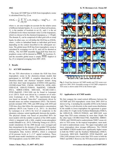
Fig. 2. Zonal bias between ACCMIP models and TES ozone averaged
Zonal over bias between 2005–2010. ACCMIP Ensemble models andaverage TES ozone of averaged ACCMIP over compared 2005-2010. toEnsemble
averageTES of ACCMIP ozonecompared is showntounder TES ozone ENSis in shown theunder bottom ENSright.
in the bottom
Fig. 2:
right.
5.2 Application to ACCMIP models
25
We first compare the zonal-vertical difference between the
ACCMIP and TES tropospheric ozone from 2005–2010 as
shown in Fig. 2 including the ensemble (ENS) in the bottom
right. There is a rich diversity in the zonal ozone distribution.
In the middle to lower troposphere the agreement is generally
within 10–15 ppb. In the Northern Midlatitudes (NMLT),
the GISS-E2-R, GISS-E2-TOMAS, and MOCAGE were
larger than TES ozone estimates by more than 10 ppb. On
the other hand, CICERO-OsloCTM2, HadGEM2, MIROC-
CHEM, and CMAM tend to underestimate NMLT ozone relative
to TES ozone. In the tropical troposphere, most models
tend to underestimate ozone. The upper troposphere and
lower stratosphere show stronger differences. The CMAM
and MIROC-CHEM models have significantly higher ozone
in both the NMLT and the Southern Midlatitudes (SMLT).
Conversely, MOCAGE, HadGEM2, STOC-HadAM3, and
UM-CAM estimate lower ozone than TES ozone in both the
NMLT and SMLT. However, the TES observation operator is
Atmos. Chem. Phys., 13, 4057–4072, 2013
www.atmos-chem-phys.net/13/4057/2013/